#78 in a series of articles about the technology behind Bang & Olufsen loudspeakers
Almost all sound systems offer bass and treble adjustments for the sound – these are basically coarse versions of a more general tool called an equaliser that is often used in recording studios, and are increasingly found in high-end home audio equipment.
Once upon a time, if you made a long-distance phone call, there was an actual physical connection made between the wire running out of your telephone and the telephone at the other end of the line. This caused a big problem in signal quality because a lot of high-frequency components of the signal would get attenuated along the way due to losses in the wiring. Consequently, booster circuits were made to help make the relative levels of the various frequencies more equal. As a result, these circuits became known as equalisers. Nowadays, of course, we don’t need to use equalisers to fix the quality of long-distance phone calls (mostly because the communication paths use digital encoding instead of analogue transmission), but we do use them to customise the relative balance of various frequencies in an audio signal. This happens most often in a recording studio, but equalisers can be a great personalisation tool in a playback system in the home.
The two main reasons for using equalisation in a playback system are (1) personal preference and (2) compensation for the effects of the listening room’s acoustical behaviour.
Equalisers are typically comprised of a collection of filters, each of which has up to 4 “handles” or “parameters” that can be manipulated by the user. These parameters are
- Filter Type
- Gain
- Centre Frequency
- Q
Filter Type
The filter type will let you decide the relative levels of signals at frequencies within the band that you’re affecting.
There are up to 7 different types of filters that can be found in professional parametric equalisers. These are (in no particular order…)
- Low Pass
- High Pass
- Low shelving
- High shelving
- Band-pass
- Band-reject
- Peaking (also known as Peak/Dip or Peak/Notch)
However, for this posting, we’ll just focus on the three most-used of these:
- Low shelving
- High shelving
- Peaking
Low Shelving Filter
In theory, a low shelving filter affects gain of all frequencies below the stated frequency by the same amount. In reality, there is a band around the stated frequency where the filter transitions between a gain of 0 dB (no change in the signal) and the gain of the affected frequency band.


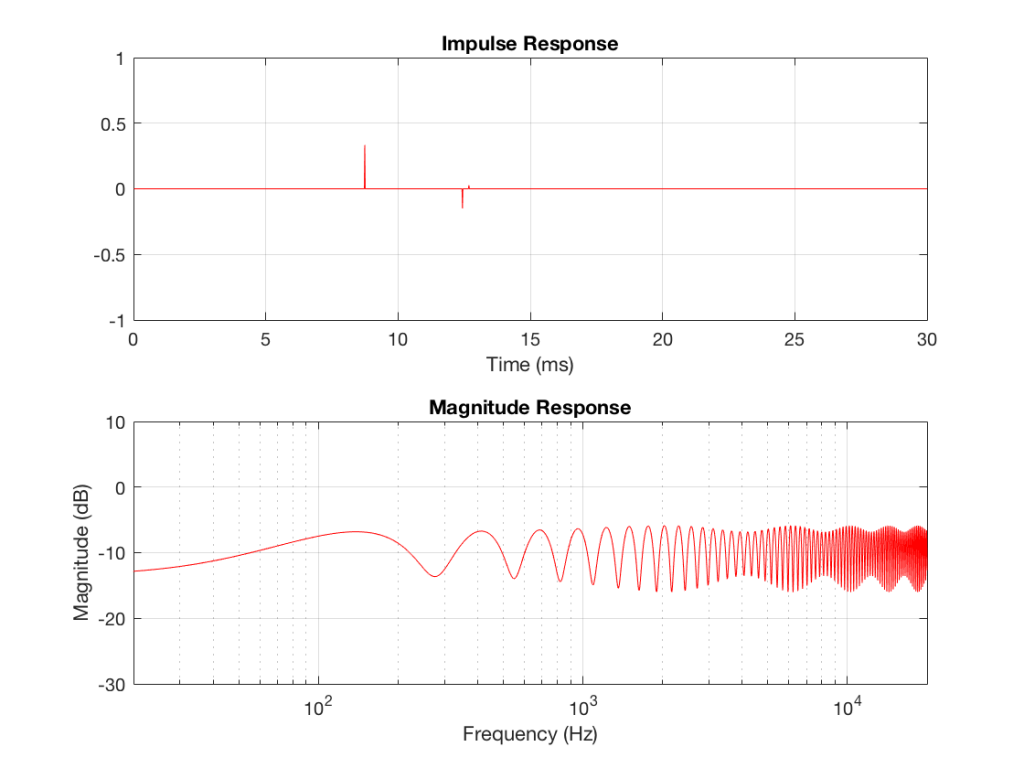
Note that the low shelving filters used in the parametric equalisers in Bang & Olufsen loudspeakers define the centre frequency as being the frequency where the gain is one half the maximum (or minimum) gain of the filter. For example, in Figure 1, the gain of the filter is 6 dB. The centre frequency is the frequency where the gain is one-half this value or 3 dB, which can be found at 80 Hz.
Some care should be taken when using low shelving filters since their affected frequency bands extend to 0 Hz or DC. This can cause a system to be pushed beyond its limits in extremely low frequency bands that are of little-to-no consequence to the audio signal. Note, however, that this is less of a concern for the B&O loudspeakers, since they are protected against such abuse.
High Shelving Filter
In theory, a high shelving filter affects gain of all frequencies above the stated frequency by the same amount. In reality, there is a band around the stated frequency where the filter transitions between a gain of 0 dB (where there is no change in the signal) and the gain of the affected frequency band.


Note again that the high shelving filters used in B&O loudspeakers define the centre frequency as being the frequency where the gain is one half the maximum (or minimum) gain of the filter. For example, in Figure 4, the gain of the filter is -6 dB. The centre frequency is the frequency where the gain is one-half this value or -3 dB, which can be found at 8 kHz.
Some care should be taken when using high shelving filters since their affected frequency bands can extend beyond the audible frequency range. This can cause a system to be pushed beyond its limits in extremely high frequency bands that are of little-to-no consequence to the audio signal.
Peaking Filter
A peaking filter is used for a more local adjustment of a frequency band. In this case, the centre frequency of the filter is affected most (it will have the Gain of the filter applied to it) and adjacent frequencies on either side are affected less and less as you move further away. For example, Figure 5 shows the response of a peaking filter with a centre frequency of 1 kHz and gains of 6 dB (the black curve) and -6 dB (the red curve). As can be seen there, the maximum effect happens at 1 kHz and frequency bands to either side are affected less.

You may notice in Figure 5 that the black and red curves are symmetrical – in other words, they are identical except in polarity (in dB) of the gain. This is a particular type of peaking filter called a reciprocal peak/dip filter – so-called because these two filters, placed in series, can be used to cancel each other’s effects on the signal.
There are other types of peaking filters that are not reciprocal. This is true in cases where the Q is defined differently. However, we won’t get into that here. If you’d like to read about this “issue”, see this link.
Gain
If you need to make all frequencies in your audio signal louder, then you just need to increase the volume. However, if you want to be a little more selective and make some frequency bands louder (or quieter) and leave other bands unchanged, then you’ll need an equaliser. So, one of the important questions to ask is “how much louder?” or “how much quieter?” The answer to this question is the gain of the filter — this is the amount by which is signal is increased or decreased in level.
The gain of an equaliser filter is almost always given in decibels or dB. (The “B” is a capital because it’s named after Alexander Graham Bell.) This is a scale based on logarithmic changes in level. Luckily, it’s not necessary to understand logarithms in order to have an intuitive feel for decibels. There are really just three things to remember:
- a gain of 0 dB is the same as saying “no change”
- positive decibel values are louder, negative decibel values are quieter
- adding approximately 6 dB to the gain is the same as saying “two times the level”. (Therefore, subtracting 6 dB is half the level.)
Centre Frequency
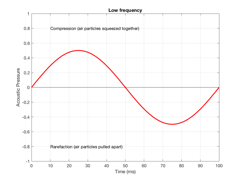
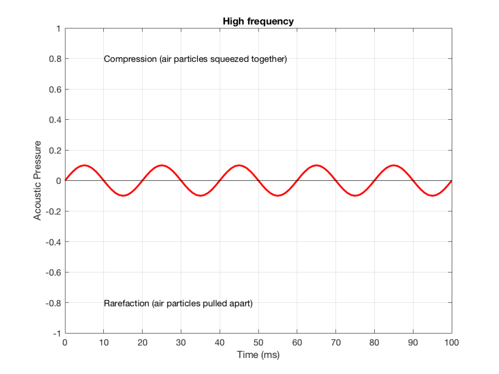
So, the next question to answer is “which frequency bands do you want to affect?” This is partially defined by the centre frequency or Fc of the filter. This is a value that is measured in the number of cycles per second (This is literally the number of times a loudspeaker driver will move in and out of the loudspeaker cabinet per second.), labelled Hertz or Hz.
Generally, if you want to increase (or reduce) the level of the bass, then you should set the centre frequency to a low value (roughly speaking, below 125 Hz). If you want to change the level of the high frequencies, then you should set the centre frequency to a high value (say, above 8 kHz).
Q
In all of the above filter types, there are transition bands — frequency areas where the filter’s gain is changing from 0 dB to the desired gain. Changing the filter’s Q allows you to alter the shape of this transition. The lower the Q, the smoother the transition. In both the case of the shelving filters and the peaking filter, this means that a wider band of frequencies will be affected. This can be seen in the examples in Figures 6 and 7.


It should be explained that the Q parameter can cause a shelving filter to behave a little strangely. When the Q of a shelving filter exceeds a value of 0.707 (or 1/sqrt(2)), the gain of the filter will “overshoot” its limits. For example, as can be seen in Figure 8, a filter with a gain of 6 dB and a Q of 4 will actually have a gain of almost 13 dB and will attenuate by almost 7 dB.

Some extra information
Some people and books will say that “Q” stands for the “Quality” of the filter. This is a very old myth, but it is not true. There is a great paper worth reading called “The Story of Q” by Estill I. Green in which it is clearly stated “His [K.S. Johnson – an employee in the Engineering Dept. of the Western Electric Company, which later became Bell Telephone Laboratories.] reason for choosing Q was quite simple. He says that it did not stand for “quality factor” or anything else, but since the other letters of the alphabet had already been pre-empted for other purposes, Q was all he had left.”
For peaking filters, the Q of the filter is equal to the centre frequency divided by the filter’s bandwidth. So, if the Q of the filter is 2 and the centre frequency is 1 kHz, then the bandwidth will be 500 Hz. Another way to look at this is that, very roughly speaking, 1/Q will be the filter’s bandwidth in octaves. So, for example, a filter with a Q of 2 will have a bandwidth of about 1/2 an octave. A filter with a Q of 0.5 will have a bandwidth of about 2 octaves.
This is just a basic introduction to parametric equalisers. For more information, check out the explanation here.