Once-upon-a-time, I taught a course in electroacoustic measurements at McGill. I used to devote an entire 3-hour class to explaining decibels, partly because we use them so often in audio, partly because I had such difficulty wrapping my own head around them when I was starting off, and partly because the reason I and many other people have that problem is largely due to the laziness of others.
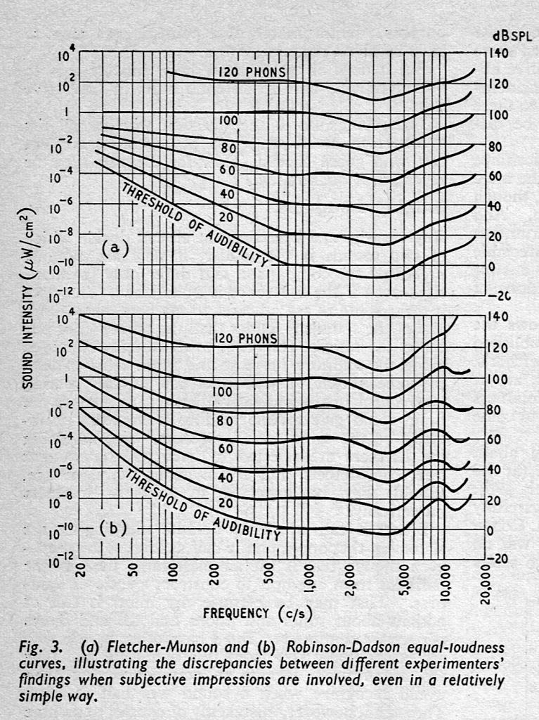
Yesterday, I found myself being annoyed once again by this laziness as I edited a scan of a document from 1961 to correct it before posting it online…
Some background information:
We humans generally respond to things logarithmically. Without getting into the math, this means that our reptile brains like multiplication more than addition.
For example: if I have $10 in the bank, and you have $100 – and we both win $10 in a lottery, I’ll be happier than you. We both won the same amount of money, but I won 100% of my current balance, whereas you only won 10% of your current balance.
Another example is a piano keyboard. Each octave looks the same distance on the keyboard, but the fundamental frequency of those notes are doubling each time you go up one octave. So, a piano keyboard (and music notation) are frequencies displayed on a logarithmic scale.
This is also true of detecting how loud things are: we think “twice as loud” or “half as loud” when talking about the Sound Pressure Level (SPL) that we hear.
We use percent and octaves to do two things:
- The first is to convert the values we’re talking about into multiplications instead of additions.
- The second is to compare a value (like our lottery winning) to another value (like the bank account balance). (It wouldn’t make sense if I said “I bought a lottery ticket and I won 100%!” 100 percent of what?)
When it comes to comparing levels of things like Sound Pressure Level, electrical power, voltages, or radio signal power, we use decibels (or dB) to make the scale logarithmic.
So, you’ll see someone write something like “the sound of a jet engine at takeoff is 120 decibels”, which is when my pet peeve rears its ugly head. The problem is that this sentence is incomplete.
If you do the math, then you find out that “120 decibels” is the same as saying “1,000,000 times” (because 10^(120/20) = 1,000,000)*, which means that the following two sentence fragments say exactly the same thing:
- “the sound of a jet engine at takeoff is 120 dB”
- “the sound of a jet engine at takeoff is 1,000,000 times louder than”
“louder than” what? THIS is the problem. The sentence should have said
“the sound of a jet engine at takeoff is 120 dB SPL” which means
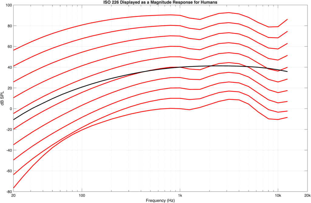
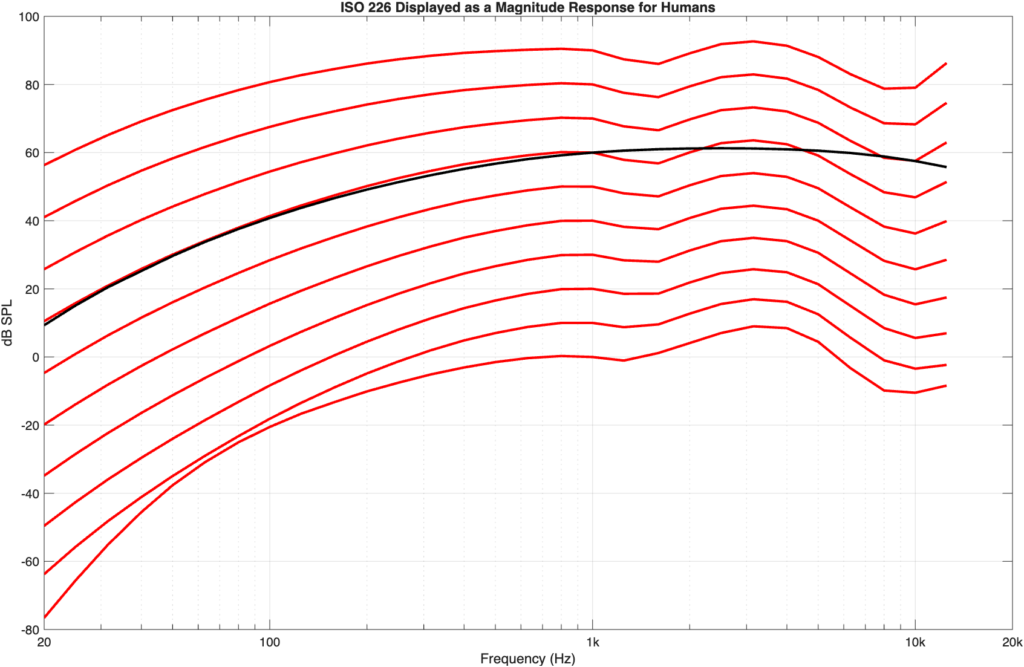
“the sound of a jet engine at takeoff is 1,000,000 times louder than the quietest level that an average person can hear when the audio signal is a 1 kHz sinusoidal tone.”
Without the “SPL” after the “dB”, there’s no way to know what you’re talking about, which is why, 40 years ago, I couldn’t understand what a “decibel” was – and why, 10 years later, my students had such trouble as well.
Without the “SPL”, it would be like if speed limits said that you should drive “50 km/”. Per second? Per minute? Per hour? Per day? These are very different things…
This also means that if you’re talking about something else, then you need a different letter after the “dB”. For example:
- Sound Pressure Level
“dB SPL” means “sound pressure level relative to a sound pressure level of 20 µPascals”
- Volts
“dB V” means “voltage relative to 1 V RMS”
- Volts (another version)
“dB u” means “voltage relative to 0.775 V RMS”
- Watts
“dB m” means “voltage relative to 1 mW”
and there are lots more…
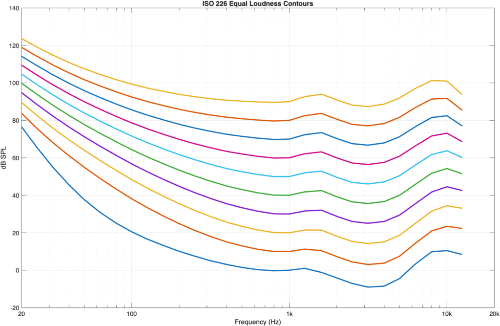
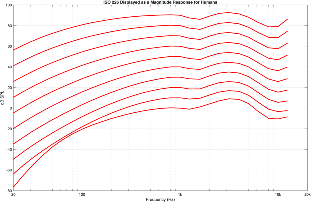
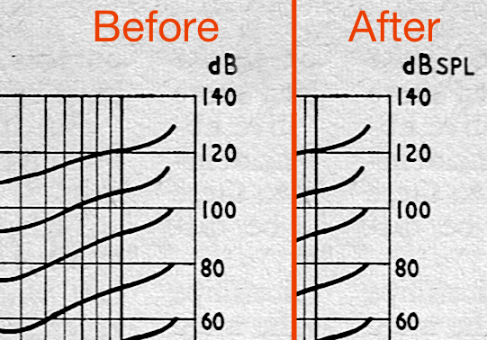
In case it’s interesting, a before-and-after of the plot that I edited yesterday is here:
… and if you want to dig into this a little more deeply, then I wrote this explanation for my electroacoustic measurements course 30 years ago
* Five last things:
#1: If you already have the measurement of the thing that you want to express in decibels relative to something else, AND it’s a pressure or voltage measurement, then the math you do is:
x dB = 20 * log10(Pressure1 / Pressure2)
For example, if Pressure1 = 2.5 pascals and Pressure2 = 1.25 pascals, then
20 * log10(2.5/1.25) = 6.02 dB
So you can say that 2.5 pascals is 6.02 decibels higher than 1.25 pascals.
If, instead, Pressure2 is the standard reference of 20 µPa, then:
20 * log10(2.5/0.00002) = 101.9
So, you can say that 2.5 pascals is 101.9 dB SPL.
#2: If you want to do it backwards for pressure or voltage then the math you do is:
Pressure2 * 10^(dB/20) = Pressure1
If you have the dB SPL value and you want to find out how many pascals you’re talking about, then Pressure2 = 0.00002
For example, if you know that the measurement is 101.9 dB SPL, then:
0.00002 * 10^(101.9 / 20) = 2.489 pascals
#3: Some examples:
- 20 * log10(4/2) = 6.02 dB
“+6 dB” is about the same as saying “times 2”
- 20 * log10(5/10) = -6.02 dB
“-6 dB” is about the same as saying “times one half”
- 20 * log10(100/10) = 20 dB
“+20 dB” is exactly the same as saying “times 10”
- 20 * log10(20/200) = -20 dB
“-20 dB” is exactly the same as saying “times 0.1”
#4: If you’re measuring power (in electrical watts or acoustic watts), then the math is slightly different.
#5: If you also see a letter in parentheses at the end such as dB SPL (A) or dB SPL (C), then this means something that you cannot ignore, but that I will not explain here…