I’ve started working with a number of my colleagues on a series of videos for internal training at Bang & Olufsen. They were kind enough to make some of these videos publicly available.
This video explains (and demonstrates) how recording engineers are able to control the perceived location of different sound sources in a two-channel stereo recording using different techniques.
One of my favourite pithy quotes is ‘Tradition is just peer pressure from dead people’. When you start looking at some of the things we ‘just do’, you start asking yourself ‘why, exactly?’
For example, when you attend a wedding, you’ll see the bride standing on the groom’s left. This is so that he can use his sword to fight off her family as he carries away from the town over his left shoulder.
Another example is the story that’s often told about how the distance between railway tracks is related to the width of a horse’s ass.
There’s a similar thing that happens in multichannel audio systems. When people ask me what I would recommend for loudspeakers when building a multichannel (or ‘surround’) system, I always start with the ITU’s Recommendation BS.775 which says that you should use matching loudspeakers all-round. Of course, almost no one does this, so the next best thing is to say something like the following:
use big loudspeakers for your Left Front and Right Front
use smaller (but matched) loudspeakers for your surround channels (including back and height channels)
make some intelligent choice about your Centre Front loudspeaker (which is not terribly helpful, but there are many issues to consider when thinking about your centre front loudspeaker)
This raises a question:
‘Why is it okay to use smaller, less capable loudspeakers for the surround channels?’
The simple answer to this is that for most materials, there isn’t as much signal in the surround channels, and there’s certainly less low-frequency, high-level content.
However, let’s keep asking questions:
‘Why isn’t there more content (in terms of both bandwidth and level) in the surround and height channels?’
The answer to this is that surround sound (like stereo, which is in effect the same thing) originated with movies. The first big blockbuster that was released in Dolby Stereo (later re-branded as Dolby Surround) was Star Wars in 1977 or so. Dolby Stereo was a 4-2-4 ‘encoding’ system that relied heavily on M-S encoding and decoding. If I over-simplify this a little, then the basic idea was:
The Centre channel was sent to both the Left and Right channels on the film
Left channel was sent to Left
Right channel was sent to Right
The Surround channel (there was only one) was mixed into the Left and Right channels in opposite polarity (aka ‘out of phase’)
So, the re-recording engineer (the film world’s version of a recording engineer) mixed in a 4-channel world: Left, Right, Centre, and Surround, but the film only contained two channels: Left Total and Right Total (with the Centre and Surround content mixed in them).
When the film was shown in a theatre with a Dolby Stereo decoder, the two channels on the film were ‘decoded’ to the original four channels and send out to the loudspeakers in the cinema.
This was a great concept based on an old idea, since M-S processing was part of Blumlein’s original patent for stereo back in 1931. When you’re looking at a two-channel stereo signal, you can think of it as independent Left and Right channels. However, usually, if you look at the content, the two channels contain related information. For example, the lead vocal of almost every pop tune is identical in the Left and Right channels so that its phantom image appears in the centre.
So, another way of thinking of the same two-channel stereo signal is by considering the two channels as
‘M’ (for Mid or Mono, depending on which book you read): the signal that is identical in the Left and Right
‘S’ (for Side or Stereo): the signal that is identical except in opposite polarity in the Left and Right
For example, FM Stereo is not sent as Left and Right channels, it’s sent as M and S channels. There’s less bandwidth and less level in the S component, so when you lose the FM signal to your antenna, the first thing to go is the S, and you’re left with a Mono radio station.
Wait… there’s that ‘less bandwidth and less level in the S component’ again – just like what I said above about the surround channels in a surround system.
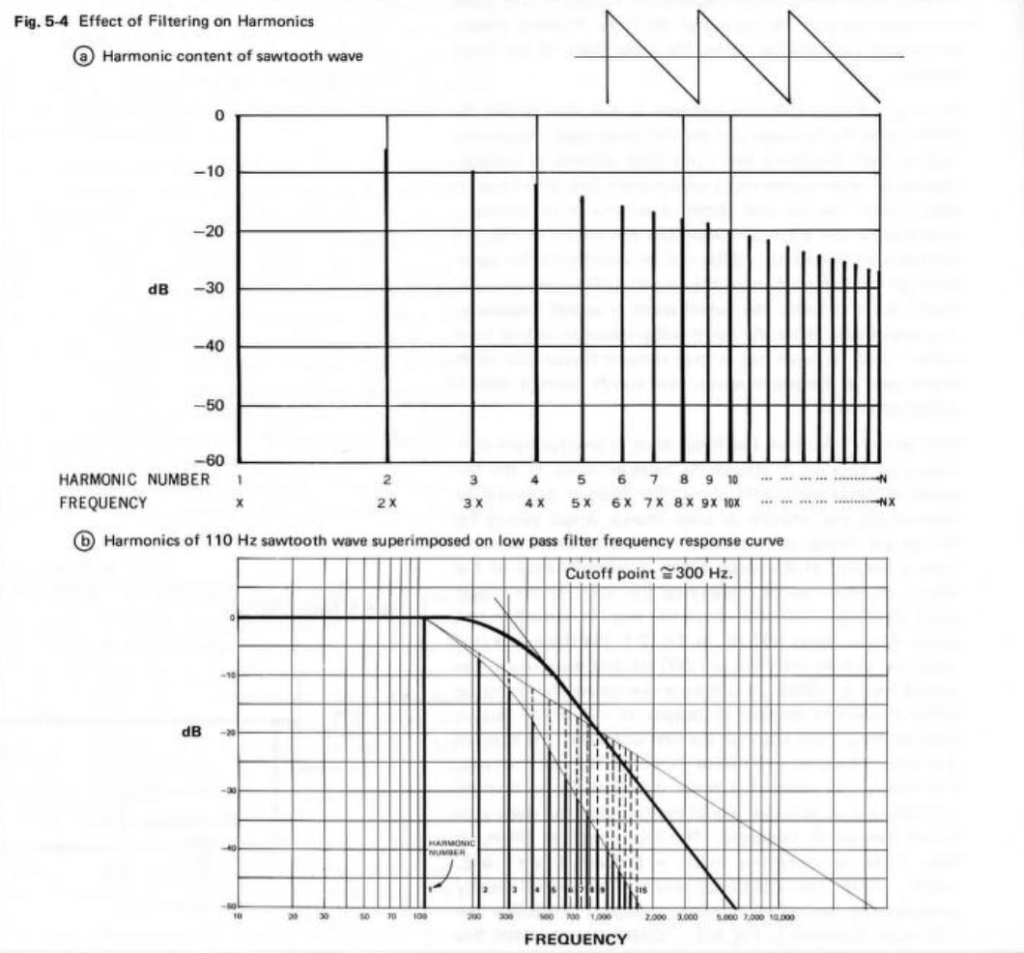
Let’s back up a little to vinyl records. A groove of a vinyl record is a 90º cut, with the needle resting gently on both walls of that trough. If the left wall moves up and down (on a 45º angle to the surface of the vinyl) then the needle bounces up and down with it, but only for that left channel. In other words, it slides along the right wall of the tough.
When a signal is the same in the left and right channels on a vinyl record (the M-component, like the lead vocal) then, when one side of the groove pushes the needle UP, the other side drops DOWN. This means that the M-component signal results in the needle moving horizontally (or laterally), in parallel with the surface of the disc. Signals in the S-component (when the Left and Right channels are ‘out of phase’) result in the two walls moving upwards and downwards together, pushing the needle vertically.
The reason for this is that the old mono shellac discs used laterally-cut grooves, and the reason for this was (apparently) that Emile Berliner was getting around a Thomas Edison patent. Also, by making the needle sensitive to lateral movements, it was less sensitive to vibrations caused by footsteps, which primarily cause the gramophone to vibrate vertically. When they made the first two-channel discs, it was smart to make the format backwards-compatible with Berliner’s existing gramophones.
So, if you have a lot of level and a lot of low-frequency content in the signal on a vinyl record, it causes the needle to jump up and down, and it will likely get thrown out of the groove and cause the record to skip. This is why the bass on vinyl records has to be monophonic, even though the record itself is two-channel stereo. Mono bass causes the needle to wiggle left-right, but not up-down.
So, the historically-accurate answer to explain why it’s okay to use smaller loudspeakers for most of the outputs in a modern 7.1.4 system is that we are maintaining compatibility with a format from 1892.
This episode of The Infinite Monkey Cage is worth a listen if you’re interested in the history of recording technologies.
There’s one comment in there by Brian Eno that I COMPLETELY agree with. He mentions that we invented a new word for moving pictures: “movies” to distinguish them from the live equivalent, “plays”. But we never really did this for music… Unless, of course, you distinguish listening to a “concert” from listening to a “recording” – but most of us just say “I’m listening to music”.
If you have a vinyl record, and you’re curious about where in the world it was pressed, this site might have some information to help you trace its roots.
Once-upon-a-time I posted a little thing about Burmese Colour Needles for grammophones. Then, today, I received an email from the owner of www.burmesecolourneedles.com a company owned by Andy Briggs, where you can buy brand new ones!
Andy also has a YouTube channel that is well worth visiting.
When you look at the datasheet of an audio device, you may see a specification that states its “signal to noise ratio” or “SNR”. Or, you may see the “dynamic range” or “DNR” (or “DR”) lists as well, or instead.
These days, even in the world of “professional audio” (whatever that means), these two things are similar enough to be confused or at least confusing, but that’s because modern audio devices don’t behave like their ancestors. So, if we look back 30 years ago and earlier, then these two terms were obviously different, and therefore independently usable. So, in order to sort this out, let’s take a look at the difference in old audio gear and the new stuff.
Let’s start with two of basic concepts:
All audio devices (or storage media or transmission systems) make noise. If you hold a resistor up in the air and look at the electrical difference across its two terminals and you’ll see noise. There’s no way around this. So, an amplifier, a DAC, magnetic tape, a digital recording stored on a hard drive… everything has some noise floor at the bottom that’s there all the time.
All audio devices have some maximum limit that cannot be exceeded. A woofer can move in and out until it goes so far that it “bottoms out” on the magnet or rips the surround. A power amplifier can deliver some amount of current, but no higher. The headphone output on your iPhone cannot exceed some voltage level.
So, the goal of any recording or device that plays a recording is to try and make sure that the audio signal is loud enough relative to that noise that you don’t notice it, but not so loud that the limit is hit.
Now we have to look a little more closely at the details of this…
If we take the example of a piece of modern audio equipment (which probably means that it’s made of transistors doing the work in the analogue domain, and there’s lots of stuff going on in the digital domain) then you have a device that has some level of constant noise (called the “noise floor”) and maximum limit that is at a very specific level. If the level of your audio signal is just a weeee bit (say, 0.1 dB) lower than this limit, then everything is as it should be. But once you hit that limit, you hit it hard – like a brick wall. If you throw your fist at a brick wall and stop your hand 1 mm before hitting it, then you don’t hit it at all. If you don’t stop your hand, the wall will stop it for you.
In older gear, this “brick wall” didn’t exist in lots of gear. Let’s take the sample of analogue magnetic tape. It also has a noise floor, but the maximum limit is “softer”. As the signal gets louder and louder, it starts to reach a point where the top and bottom of the audio waveform get increasingly “squished” or “compressed” instead of chopping off the top and bottom.
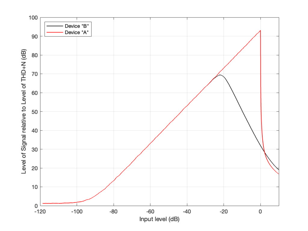
I made a 997 Hz sine wave that starts at a very, very low level and increases to a very high level over a period of 10 seconds. Then, I put it through two simulated devices.
Device “A” is a simulation of a modern device (say, an analogue-to-digital converter). It clips the top and bottom of the signal when some level is exceeded.
Device “B” is a simulation of something like the signal that would be recorded to analogue magnetic tape and then played back. Notice that it slowly “eases in” to a clipped signal; but also notice that this starts happening before Device “A” hits its maximum. So, the signal is being changed before it “has to”.
Let’s zoom in on those two plots at two different times in the ramp in level.
Device “A” is the two plots on the top at around 8.2 seconds and about 9.5 seconds from the previous figure. Device “B” is the bottom two plots, zooming in on the same two moments in time (and therefore input levels).
Notice that when the signal is low enough, both devices have (roughly) the same behaviour. They both output a sine wave. However, when the signal is higher, one device just chops off the top and bottom of the sine wave whereas the other device merely changes its shape.
Now let’s think of this in terms of the signals’ levels in relationship to the levels of the noise floors of the devices and the distortion artefacts that are generated by the change in the signals when they get too loud.
If we measure the output level of a device when the signal level is very, very low, all we’ll see is the level of the inherent noise floor of the device itself. Then, as the signal level increases, it comes up above the noise floor, and the output level is the same as the level of the signal. Then, as the signal’s level gets too high, it will start to distort and we’ll see an increase in the level of the distortion artefacts.
If we plot this as a ratio of the signal’s level (which is increasing over time) to the combined level of the distortion and noise artefacts for the two devices, it will look like this:
On the left side of this plot, the two lines (the black door Device “A” and the red for Device “B”) are horizontal. This is because we’re just seeing the noise floor of the devices. No matter how much lower in level the signals were, the output level would always be the same. (If this were a real, correct Signal-to-THD+N ratio, then it would actually show negative values, because the signal would be quieter than the noise. It would really only be 0 dB when the level of the noise was the same as the signal’s level.)
Then, moving to the right, the levels of the signals come above the noise floor, and we see the two lines increasing in level.
Then, just under a signal level of about -20 dB, we see that the level of the signal relative to the artefacts starts in Device “B” reaches a peak, and then starts heading downwards. This is because as the signal level gets higher and higher, the distortion artefacts increase in level even more.
However, Device “A” keeps increasing until it hits a level 0 dB, at which point a very small increase in level causes a very big jump in the amount of distortion, so the relative level of the signal drops dramatically (not because the signal gets quieter, but because the distortion artefacts get so loud so quickly).
Now let’s think about how best to use those two devices.
For Device “A” (in red) we want to keep the signal as loud as possible without distorting. So, we try to make sure that we stay as close to that 0 dB level on the X-axis as we can most of the time. (Remember that I’m talking about a technical quality of audio – not necessarily something that sounds good if you’re listening to music.) HOWEVER: we must make sure that we NEVER exceed that level.
However, for Device “B”, we want to keep the signal as close to that peak around -20 dB as much as possible – but if we go over that level, it’s no big deal. We can get away with levels above that – it’s just that the higher we go, the worse it might sound because the distortion is increasing.
Notice that the red line and the black line cross each other just above the 0 dB line on the X-axis. This is where the two devices will have the same level of distortion – but the distortion characteristics will be different, so they won’t necessarily sound the same. But let’s pretend that the the only measure of quality is that Y-axis – so they’re the same at about +2 dB on the X-axis.
Now the question is “What are the dynamic ranges of the two systems?” Another way to ask this question is “How much louder is the loudest signal relative to the quietest possible signal for the two devices?” The answer to this is “a little over 100 dB” for both of them, since the two lines have the same behaviour for low signals and they cross each other when the signal is about 100 dB above this (looking at the X-axis, this is the distance between where the two lines are horizontal on the left, and where they cross each other on the right). Of course, I’m over-simplifying, but for the purposes of this discussion, it’s good enough.
The second question is “What are the signal-to-noise ratios of the two systems?” Another way to ask THIS question is “How much louder is the average signal relative to the quietest possible signal for the two devices?” The answer to this question is two different numbers.
Device “A” has a signal-to-noise ratio of about 100 dB , because we’re going to use that device, trying to keep the signal as close to clipping as possible without hitting that brick wall. In other words, for Device “A”, the dynamic range and the signal-to-noise ratio are the same because of the way we use it.
Device “B” has a signal-to-noise ratio of about 80 dB because we’re going to try to keep the signal level around that peak on the black curve (around -20 dB on the X-axis). So, its signal-to-noise ratio is about 20 dB lower than its dynamic range, again, because of the way we use it.
The problem is, these days, a lot of engineers aren’t old enough to remember the days when things behaved like Device “B”, so they interchange Signal to Noise and Dynamic Range all willy-nilly. Given the way we use audio devices today, that’s okay, except when it isn’t.
For example, if you’re trying to connect a turntable (which plays vinyl records that are mastered to behave more like Device “B”) to a digital audio system, then the makers of those two systems and the recordings you play might not agree on how loud things should be. However, in theory, that’s the problem of the manufacturers, not the customers. In reality, it becomes the problem of the customers when they switch from playing a record to playing a digital audio stream, since these two worlds treat levels differently, and there’s no right answer to the problem. As a result, you might need to adjust your volume when you switch sources.
This episode of 99 Percent Invisible tells the story of the Recording Ban of 1942, the impact on the rise of modern jazz music, and the parallels with the debates between artists and today’s streaming services. It’s worth the 50 minutes and 58 seconds it takes to listen to this!
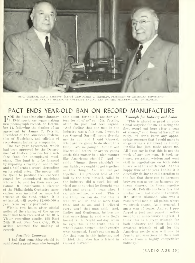
At the end of that episode, the ban on record manufacture is mentioned, almost as an epilogue. This page from the January, 1949 issue of RCA’s “Radio Age” magazine discusses the end of that ban.
Interestingly, that same issue of the magazine has an article that introduces a new recording format: 7-inch records operating at 45 revolutions per minute! The article claims that the new format is “distortion free” and “noise-free”, stating that this “new record and record player climax more than 10 years of research and refinement in this field by RCA.”


.jpg)