As was discussed in Part 3, when a record master is cut on a lathe, the cutter head follows a straight-line path as it moves from the outer rim to the inside of the disk. This means that it is always modulating in a direction that is perpendicular to the groove’s relative direction of travel, regardless of its distance from the centre.
The direction of travel of the cutting head when the master disk is created on a lathe.
A turntable should be designed to ensure that the stylus tracks the groove made by the cutter head in all aspects. This means that this perpendicular angle should be maintained across the entire surface of the disk. However, in the case of a tonearm that pivots, this is not possible, since the stylus follows a circular path, resulting in an angular tracking error.
Any tonearm has some angular tracking error that varies with position on the disk.
The location of the pivot point, the tonearm’s shape, and the mounting of the cartridge can all contribute to reducing this error. Typically, tonearms are designed so that the cartridge is angled to not be in-line with the pivot point. This is done to ensure that there can be two locations on the record’s surface where the stylus is angled correctly relative to the groove.
A correctly-designed and aligned pivoting tonearm has a tracking error of 0º at only two locations on the disk.
However, the only real solution is to move the tonearm in a straight line across the disc, maintaining a position that is tangential to the groove, and therefore keeping the stylus located so that its movement is perpendicular to the groove’s relative direction of travel, just as it was with the cutter head on the lathe.
A tonearm that travels sideways, maintaining an angle that is tangent to the groove at the stylus.
In a perfect system, the movement of the tonearm would be completely synchronous with the sideways “movement” of the groove underneath it, however, this is almost impossible to achieve. In the Beogram 4000c, a detection system is built into the tonearm that responds to the angular deviation from the resting position. The result is that the tonearm “wiggles” across the disk: the groove pulls the stylus towards the centre of the disk for a small distance before the detector reacts and moves the back of the tonearm to correct the angle.
Typically, the distance moved by the stylus before the detector engages the tracking motor is approximately 0.1 mm, which corresponds to a tracking error of approximately 0.044º.
An exaggerated representation of the maximum tracking error of the tonearm before the detector engages and corrects.
One of the primary artefacts caused by an angular tracking error is distortion of the audio signal: mainly second-order harmonic distortion of sinusoidal tones, and intermodulation distortion on more complex signals. (see “Have Tone Arm Designers Forgotten Their High-School Geometry?” in The Audio Critic, 1:31, Jan./Feb., 1977.) It can be intuitively understood that the distortion is caused by the fact that the stylus is being moved at a different angle than that for which it was designed.
It is possible to calculate an approximate value for this distortion level using the following equation:
Where is the harmonic distortion in percent, is the angular frequency of the modulation caused by the audio signal (calculated using ), is the peak amplitude in mm, is the tracking error in degrees, is the angular frequency of rotation (the speed of the record in radians per second. For example, at 33 1/3 RPM, ) and is the radius (the distance of the groove from the centre of the disk). (see “Tracking Angle in Phonograph Pickups” by B.B. Bauer, Electronics (March 1945))
This equation can be re-written, separating the audio signal from the tonearm behaviour, as shown below.
which shows that, for a given audio frequency and disk rotation speed, the audio signal distortion is proportional to the horizontal tracking error over the distance of the stylus to the centre of the disk. (This is the reason one philosophy in the alignment of a pivoting tonearm is to ensure that the tracking error is reduced when approaching the centre of the disk, since the smaller the radius, the greater the distortion.)
It may be confusing as to why the position of the groove on the disk (the radius) has an influence on this value. The reason is that the distortion is dependent on the wavelength of the signal encoded in the groove. The longer the wavelength, the lower the distortion. As was shown in Figure 1 in Part 6 of this series, the wavelength of a constant frequency is longer on the outer groove of the disk than on the inner groove.
Using the Beogram 4000c as an example at its worst-case tracking error of 0.044º: if we have a 1 kHz sine wave with a modulation velocity of 34.1 mm/sec on a 33 1/3 RPM LP on the inner-most groove then the resulting 2nd-harmonic distortion will be 0.7% or about -43 dB relative to the signal. At the outer-most groove (assuming all other variables remain constant), the value will be roughly half of that, at 0.3% or -50 dB.
In order to keep the stylus tip in the groove of the record, it must have some force pushing down on it. This force must be enough to keep the stylus in the groove. However, if it is too large, then both the vinyl and the stylus will wear more quickly. Thus a balance must be found between “too much” and “not enough”.
Figure 1: Typical tracking force over time. The red portion of the curve shows the recommendation for Beogram 4002 and Beogram 4000c.
As can be seen in Figure 1, the typical tracking force of phonograph players has changed considerably since the days of gramophones playing shellac discs, with values under 10 g being standard since the introduction of vinyl microgroove records in 1948. The original recommended tracking force of the Beogram 4002 was 1 g, however, this has been increased to 1.3 g for the Beogram 4000c in order to help track more recent recordings with higher modulation velocities and displacements.
Effective Tip Mass
The stylus’s job is to track all of the vibrations encoded in the groove. It stays in that groove as a result of the adjustable tracking force holding it down, so the moving parts should be as light as possible in order to ensure that they can move quickly. The total apparent mass of the parts that are being moved as a result of the groove modulation is called the effective tip mass. Intuitively, this can be thought of as giving an impression of the amount of inertia in the stylus.
It is important to not confuse the tracking force and the effective tip mass, since these are very different things. Imagine a heavy object like a 1500 kg car, for example, lifted off the ground using a crane, and then slowly lowered onto a scale until it reads 1 kg. The “weight” of the car resting on the scale is equivalent to 1 kg. However, if you try to push the car sideways, you will obviously find that it is more difficult to move than a 1 kg mass, since you are trying to overcome the inertia of all 1500 kg, not the 1 kg that the scale “sees”. In this analogy, the reading on the scale is equivalent to the Tracking Force, and the mass that you’re trying to move is the Effective Tip Mass. Of course, in the case of a phonograph stylus, the opposite relationship is desirable; you want a tracking force high enough to keep the stylus in the groove, and an effective tip mass as close to 0 as possible, so that it is easy for the groove to move it.
Compliance
Imagine an audio signal that is on the left channel only. In this case, the variation is only on one of the two groove walls, causing the stylus tip to ride up and down on those bumps. If the modulation velocity is high, and the effective tip mass is too large, then the stylus can lift off the wall of the groove just like a car leaving the surface of a road on the trailing side of a bump. In order to keep the car’s wheels on the road, springs are used to push them back down before the rest of the car starts to fall. The same is true for the stylus tip. It’s being pushed back down into the groove by the cantilever that provides the spring. The amount of “springiness” is called the compliance of the stylus suspension. (Compliance is the opposite of spring stiffness: the more compliant a spring is, the easier it is to compress, and the less it pushes back.)
Like many other stylus parameters, the compliance is balanced with other aspects of the system. In this case it is balanced with the effective mass of the tonearm (which includes the tracking force(1), resulting in a resonant frequency. If that frequency is too high, then it can be audible as a tone that is “singing along” with the music. If it’s too low, then in a worst-case situation, the stylus can jump out of the record groove.
If a turntable is very poorly adjusted, then a high tracking force and a high stylus compliance (therefore, a “soft” spring) results in the entire assembly sinking down onto the record surface. However, a high compliance is necessary for low-frequency reproduction, therefore the maximum tracking force is, in part, set by the compliance of the stylus.
If you are comparing the specifications of different cartridges, it may be of interest to note that compliance is often expressed in one of five different units, depending on the source of the information:
“Compliance Unit” or “cu”
mm/N millimetres of deflection per Newton of force
µm/mN micrometres of deflection per thousandth of a Newton of force
x 10^-6 cm/dyn hundredths of a micrometre of deflection per dyne of force
x 10^-6 cm / 10^-5 N hundredths of a micrometre of deflection per hundred-thousandth of a Newton of force
Since
mm/N = 1000 µm / 1000 mN
and
1 dyne = 0.00001 Newton
Then this means that all five of these expressions are identical, so, they can be interchanged freely. In other words:
The earliest styli were the needles that were used on 78 RPM gramophone players. These were typically made from steel wire that was tapered to a conical shape, and then the tip was rounded to a radius of about 150 µm, by tumbling them in an abrasive powder.(1) This rounded curve at the tip of the needle had a hemispherical form, and so styli with this shape are known as either conical or spherical.
The first styli made for “microgroove” LP’s had the same basic shape as the steel predecessor, but were tipped with sapphire or diamond. The conical/spherical shape was a good choice due to the relative ease of manufacture, and a typical size of that spherical tip was about 36 µm in diameter. However, as recording techniques and equipment improved, it was realised that there are possible disadvantages to this design.
Remember that the side-to-side shape of the groove is a physical representation of the audio signal: the higher the frequency, the smaller the wave on the disc. However, since the disc has a constant speed of rotation, the speed of the stylus relative to the groove is dependent on how far away it is from the centre of the disc. The closer the stylus gets to the centre, the smaller the circumference, so the slower the groove speed.
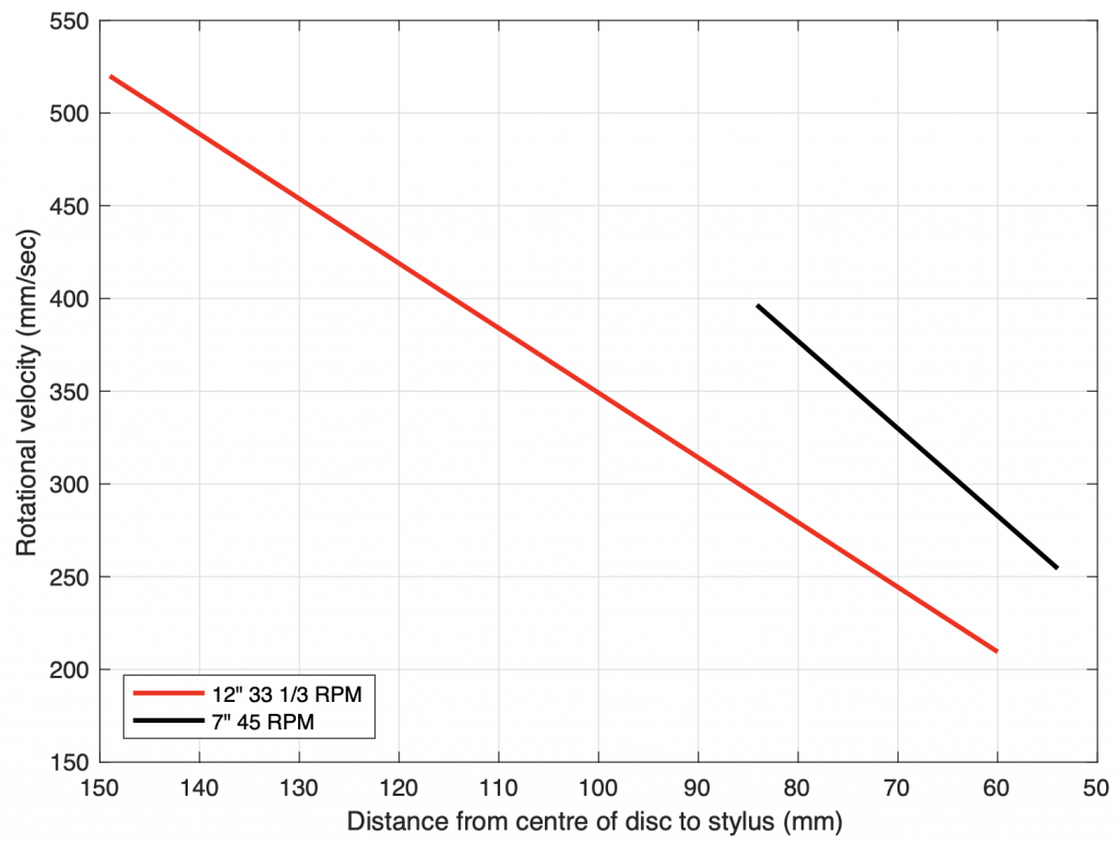
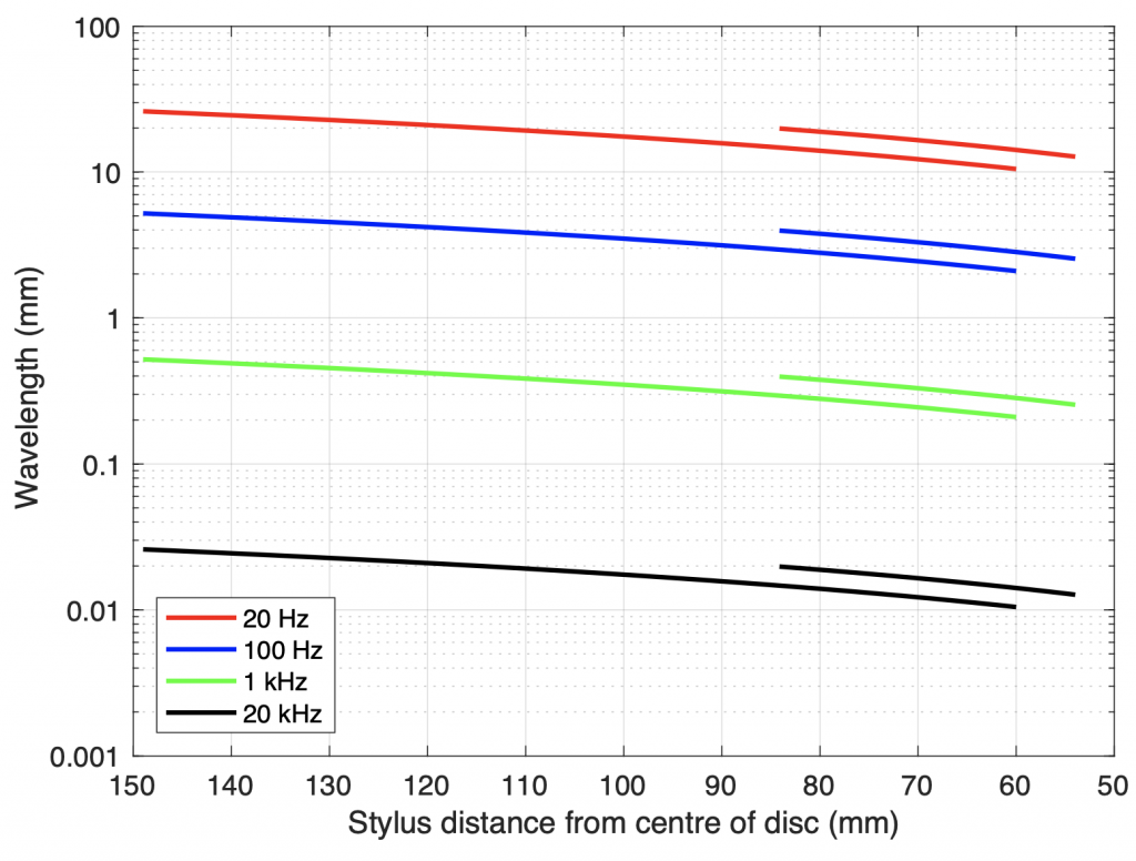
If we look at a 12″ LP, the smallest allowable diameter for the modulated groove is about 120 mm, which gives us a circumference of about 377 mm (or 120 * π). The disc is rotating 33 1/3 times every minute which means that it is making 0.56 of a rotation per second. This, in turn, means that the stylus has a groove speed of 209 mm per second. If the audio signal is a 20,000 Hz tone at the end of the recording, then there must be 20,000 waves carved into every 209 mm on the disc, which means that each wave in the groove is about 0.011 mm or 11 µm long.
Figure 1: The relative speed of the stylus to the surface of the vinyl as it tracks from the outside to the inside radius of the record.Figure 2: The wavelengths measured in the groove, as a function of the stylus’s distance to the centre of a disc. The shorter lines are for 45 RPM 7″discs, the longer lines are for 33 1/3 RPM 12″ LPs.
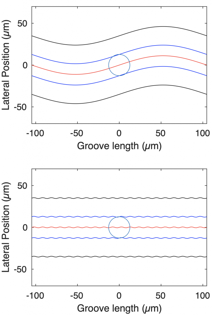
However, now we have a problem. If the “wiggles” in the groove have a total wavelength of 11 µm, but the tip of the stylus has a diameter of about 36 µm, then the stylus will not be able to track the groove because it’s simply too big (just like the tires of your car do not sink into every small crack in the road). Figure 3 shows to-scale representations of a conical stylus with a diameter of 36 µm in a 70 µm-wide groove on the inside radius of a 33 1/3 RPM LP (60 mm from the centre of the disc), viewed from above. The red lines show the bottom of the groove and the black lines show the edge where the groove meets the surface of the disc. The blue lines show the point where the stylus meets the groove walls. The top plot is a 1 kHz sine wave and the bottom plot is a 20 kHz sine wave, both with a lateral modulation velocity of 70 mm/sec. Notice that the stylus is simply too big to accurately track the 20 kHz tone.
Figure 3: Scale representations of a conical stylus with a diameter of 36 µm in a 70 µm-wide groove on the inside radius of a 33 1/3 RPM LP, looking directly downwards into the groove. See the text for more information.
One simple solution was to “sharpen” the stylus; to make the diameter of the spherical tip smaller. However, this can cause two possible side effects. The first is that the tip will sink deeper into the groove, making it more difficult for it to move independently on the two audio channels. The second is that the point of contact between the stylus and the vinyl becomes smaller, which can result in more wear on the groove itself because the “footprint” of the tip is smaller. However, since the problem is in tracking the small wavelength of high-frequency signals, it is only necessary to reduce the diameter of the stylus in one dimension, thus making the stylus tip elliptical instead of conical. In this design, the tip of the stylus is wide, to sit across the groove, but narrow along the groove’s length, making it small enough to accurately track high frequencies. An example showing a 0.2 mil x 0.7 mil (10 x 36 µm) stylus is shown in Figure 4. Notice that this shape can track the 20 kHz tone more easily, while sitting at the same height in the groove as the conical stylus in Figure 3.
Figure 4: Scale representations of an elliptical stylus with diameters of 10 x 36 µm in a 70 µm-wide groove on the inside radius of a 33 1/3 RPM LP, looking directly downwards into the groove. See the text for more information.
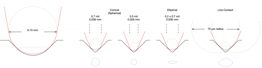
Both the conical and the elliptical stylus designs have a common drawback in that the point of contact between the tip and the groove wall is extremely small. This can be seen in Figure 5, which shows various stylus shapes from the front. Notice the length of the contact between the red and black lines (the stylus and the groove wall). As a result, both the groove of the record and the stylus tip will wear over time, generally resulting in an increasing loss of high frequency output. This was particularly a problem when the CD-4 Quadradisc format was introduced, since it relies on signals as high as 45 kHz being played from the disc.(2) In order to solve this problem, a new stylus shape was invented by Norio Shibata at JVC in 1973. The idea behind this new design is that the sides of the stylus are shaped to follow a much larger-radius circle than is possible to fit into the groove, however, the tip has a small radius like a conical stylus. An example showing this general concept can be seen on the right side of Figure 5.
Figure 5: Dimensions of example styli, drawn to scale. The figure on the left is typical for a 78 RPM steel needle. The four examples on the right show different examples of tip shapes. These are explained in more details in the text. (For comparison, a typical diameter of a human hair is about 0.06 mm.)
There have been a number of different designs following Shibata’s general concept, with names such as MicroRidge (which has an interesting, almost blade-like shape “across” the groove), Fritz-Geiger, Van-den-Hul, and Optimized Contour Contact Line. Generally, these designs have come to be known as line contact (or contact line) styli, because the area of contact between the stylus and the groove wall is a vertical line rather than a single point.
In 1973, Bang and Olufsen started working its own turntable that could play the new CD-4 Quadradisc format. This not only meant developing a new decoder with a 4-channel output, but also a stylus with a bandwidth reliably extending to approximately 45 kHz. This task was given to Villy Hansen, who was project manager for pickup development, despite being still relatively new to the company. Hansen proposed an improvement upon the Shibata grind (which was already commercially available by then) by making 4 facets instead of 2, resulting in a better shape for tracking the very high-frequency modulation. Although developed by Hansen, the new stylus became known as the “Pramanik diamond”, named after Subir K. Pramanik, who had started working as an engineer in Struer in 1971, but who had temporarily returned to India. The end result was a new pickup family that was initially launched with the top model, the MMC 6000.
Figure 6: An example of an elliptical stylus on the left vs. a line contact Pramanik grind on the right. Notice the difference in the area of contact between the styli and the groove walls.
Bonded vs. Nude
There is one small, but important point regarding a stylus’s construction. Although the tip of the stylus is almost always made of diamond today, in lower-cost units, that diamond tip is mounted or bonded to a titanium or steel pin which is, in turn, connected to the cantilever (the long “arm” that connects back to the cartridge housing). This bonded design is cheaper to manufacture, but it results in a high mass at the stylus tip, which means that it will not move easily at high frequencies.
Figure 7: Scale models (on two different scales) of different styli. The example on the left is bonded, the other four are nude.
In order to reduce mass, the steel pin is eliminated, and the entire stylus is made of diamond instead. This makes things more costly, but reduces the mass dramatically, so it is preferred if the goal is higher sound performance. This design is known as a nude stylus.
Footnotes
See “The High-fidelity Phonograph Transducer” B.B. Bauer, JAES 1977 Vol 25, Number 10/11, Oct/Nov 1977
The CD4 format used a 30 kHz carrier tone that was frequency-modulated ±15 kHz. This means that the highest frequency that should be tracked by the stylus is 30 kHz + 15 kHz = 45 kHz.
As mentioned above, when a wire is moved through a magnetic field, a current is generated in a wire that is proportional to the velocity of the movement. In order to increase the output, the wire can be wrapped into a coil, effectively lengthening the piece of wire moving through the field. Most phono cartridges make use of this behaviour by using the movement of the stylus to either:
move tiny magnets that are placed near coils of wire (a Moving Magnet or MM design or
move tiny coils of wire that are placed near very strong magnets (a Moving Coil or MC design)
In either system, there is a relative physical movement that is used to generate the electrical signal from the cartridge. There are advantages and disadvantages associated with both of these systems, however, they’re well-discussed in other places, so I won’t talk about them here.
There is a third, less common design called a Moving Iron (or variable-reluctance(1)) system, which can be thought of as a variant of the Moving Magnet principle. In this design, the magnet and the coils remain stationary, and the stylus moves a small piece of iron instead. That iron is placed between the north and south poles of the magnet so that, when it moves, it modulates (or varies) the magnetic field. As the magnetic field modulates, it moves relative to the coils, and an electrical signal is generated. One of the first examples of this kind of pickup was the Western Electric 4A reproducer made in 1925.
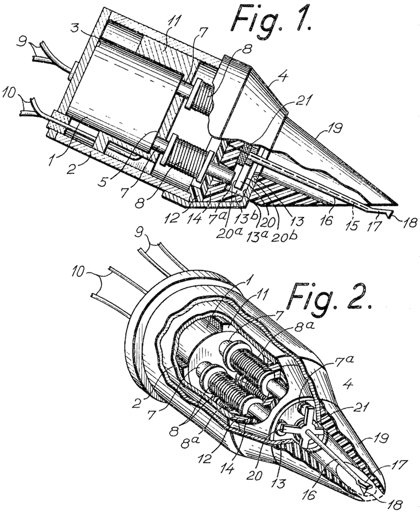
Figure 1: Figures from Rørbaek Madsen’s 1963 patent for a Stereophonic Transducer Cartridge.
In 1963, Erik Rørbaek Madsen of Bang & Olufsen filed a patent for a cartridge based on the Moving Iron principle. In it, a cross made of Mu-metal is mounted on the stylus. Each arm of the cross is aligned with the end of a small rod called a “pole piece” (because it was attached to the pole of a magnet on the opposite end). The cross is mounted diagonally, so the individual movements of the left and right channels on the groove cause the arms of the cross to move accordingly. For a left-channel signal, the bottom left and top right cross arms move in opposite directions – one forwards and one backwards. For a right-channel signal, the bottom right and top left arms move instead. The two coils that generate the current for each audio channel are wired in a push-pull relationship.
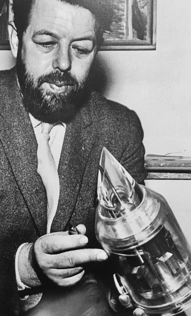
Figure 2: Erik Rørbaek Madsen explaining the MMC concept.
There are a number of advantages to this system over the MM and MC designs. Many of these are described in the original 1963 patent, as follows:
“The channel separation is very good and induction of cross talk from one channel to the other is minimized because cross talk components are in phase in opposing coils.”
“The moving mass which only comprises the armature and the stylus arm can be made very low which results in good frequency response.”
“Hum pick-up is very low due to the balanced coil construction”
“… the shielding effect of the magnetic housing … provides a completely closed magnetic circuit which in addition to shielding the coil from external fields prevents attraction to steel turntables.”
Finally, (although this is not mentioned in the patent) the push-pull wiring of the coils “reduces harmonic distortion induced by the non-linearity of the magnetic field.”(2)
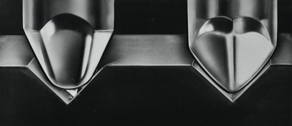
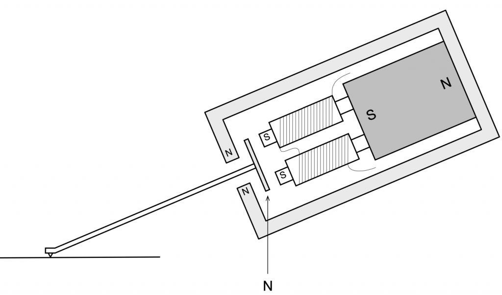
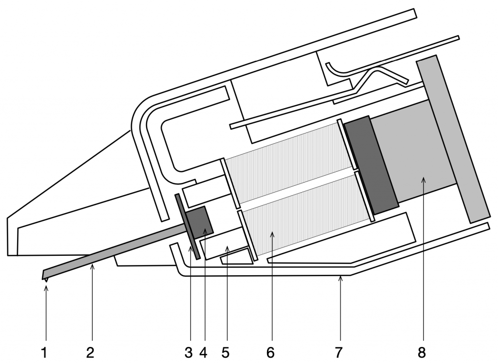
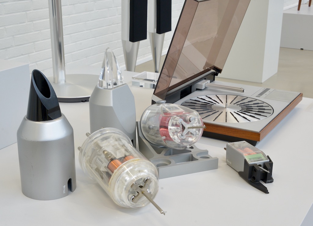
Figure 3: The magnetic circuit representation of the MMC cartridge, showing the diagonal pair of pole pieces for one of the two audio channels.Figure 4: The Micro Moving Cross MMC 4000 cartridge design. 1. Nude Pramanik diamond, 2. Low mass beryllium cantilever, 3. Moving micro cross, 4. Block suspension, 5. Pole pieces, 6. Induction coils, 7. Mu-metal screen, 8. Hycomax magnetFigure 5: Large-scale models of the MMC cartridges used for past demonstrations.
Footnotes
reluctance is the magnetic equivalent of electrical resistance
Lately, a large part of my day job has been involved with the Beogram 4000c project at Bang & Olufsen. This turned out to be pretty fun, because, as I’ve been telling people, I’m old enough that many of my textbooks have chapters about vinyl and phonographs, but I’m young enough that I didn’t have to read them, since vinyl was a dying technology in the 1990’s.
So, one I the things I’ve had to do lately is to go back and learn all the stuff I didn’t have to do 25 years ago. In the process, I’ve wound up gathering lots of information that might be of interest to someone else, so I figured I’d collect it here in a multi-part series on phonographs.
A warning: this will not be a tome on why vinyl is better than digital or why digital is better than vinyl. I’m not here to start any arguments or rail against anyone’s religious beliefs. If you don’t like some of the stuff I say here, put your complaints in your own website.
Also, if you’ve downloaded the Technical Sound Guide for the Beogram 4000c, then you’ll recognise a large portions of these postings as auto-plagiarism. Consider the TGS as a condensed version of this series.
A very short history
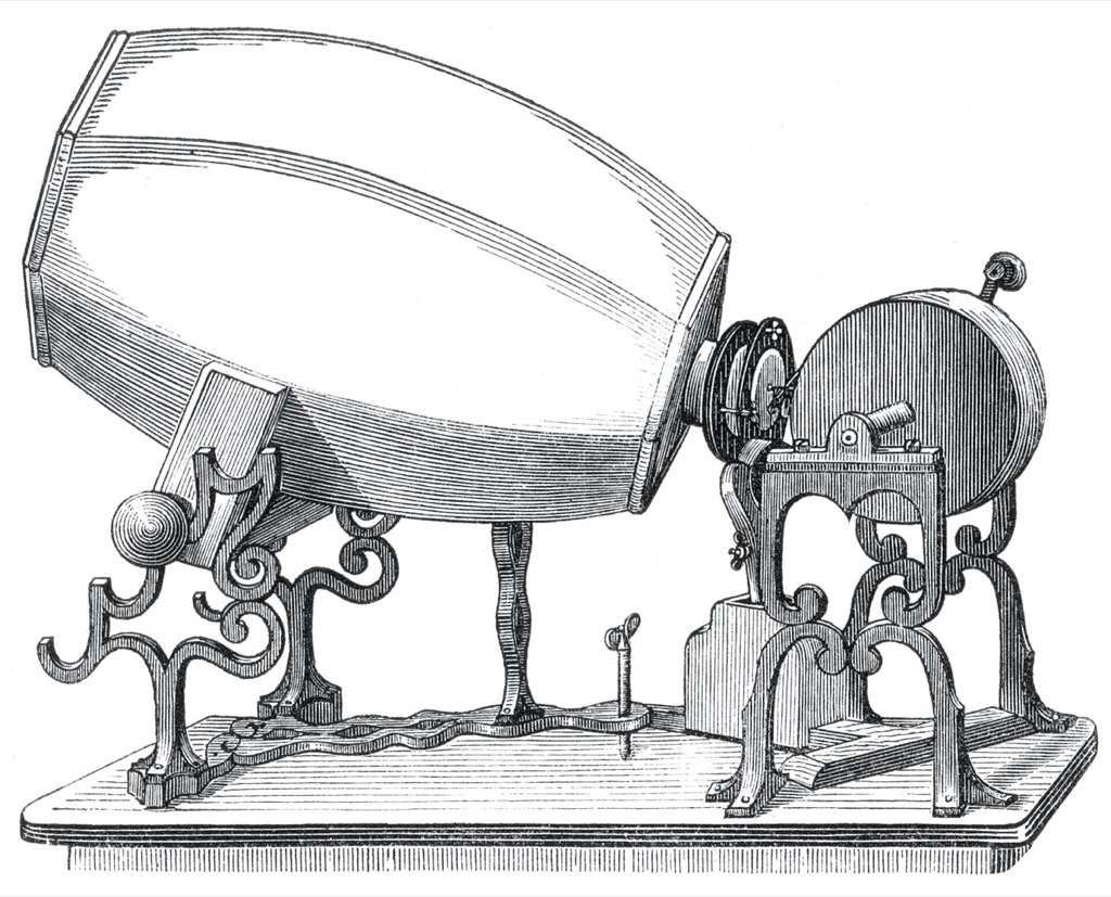
In 1856, Édouard-Léon Scott de Martinville invented a device based on the basic anatomy of the human ear. It consisted of a wooden funnel ending at a flexible membrane to emulate the ear canal and eardrum. Connected to the membrane was a pig bristle that moved with it, scratching a thin line into soot on a piece of paper wrapped around a rotating cylinder. He called this new invention a “phonautograph” or “self-writer of sound”.
The phonoautograph (from www.firstsounds.org)
This device was conceived to record sounds in the air without any intention of playing them back, so it can be considered to be the precursor to the modern oscilloscope. (It should be said that some “recordings” made on a phonoautograph were finally played in 2008. See www.firstsounds.org for more information.) However, in the late 1870’s, Charles Cros realised that if the lines drawn by the phonoautograph were photo-engraved onto the surface of a metal cylinder, then it could be used to vibrate a needle placed in the resulting groove. Unfortunately, rather than actually build such a device, he only wrote about the idea in a document that was filed at the Académie des Sciences and sealed. Within 6 months of this, in 1877, Thomas Edison asked his assistant, John Kruesi, to build a device that could not only record sound (as an indentation in tin foil on a cylinder) but reproduce it, if only a few times before the groove became smoothed. (see “Reproduction of Sound in High-fidelity and Stereo Phonographs” (1962) by Edgar Villchur)
It was ten years later, in 1887, that the German-American inventor Emil Berliner was awarded a patent for a sound recording and reproducing system that was based on a groove in a rotating disc (rather than Edison’s cylinder); the original version of the system that we know of today as the “Long Playing” or “LP” Record.
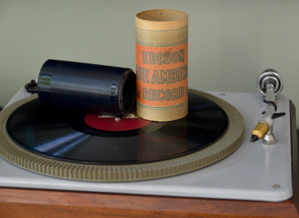
An Edison “Blue Amberol” record with a Danish 78 RPM “His Master’s Voice” disc recording X8071 of Den Blaa Anemone.
Early phonographs or “gramophones” were purely mechanical devices. The disc (or cylinder) was rotated by a spring-driven clockwork mechanism and the needle or stylus rested in the passing groove. The vibrations of the needle were transmitted to a flexible membrane that was situated at the narrow end of a horn that amplified the resulting sound to audible levels.
Magnets and Coils
In 1820, more than 30 years before de Martinville’s invention, the Danish physicist and chemist, Hans Christian Ørsted announced the first link made between electricity and magnetism: he had discovered that a compass needle would change direction when placed near a wire that was carrying an electrical current. Nowadays, it is well-known that this link is bi-directional. When current is sent through a wire, a magnetic field is generated around it. However, it is also true that moving a wire through a magnetic field will generate current that is proportional to its velocity.
This week, I was asked a very specific question about connecting an older pair of Beolab loudspeakers to a stereo preamp from another company. Specifically, the owner was wondering why the pairing wasn’t working out too well – and he had already had a theory that the problem had something to do with the sensitivity of his Beolab 9’s.
To be honest, I don’t really know what the problem is with this specific customer’s system – but I made a guess and I figured that the answer might be useful to someone else…
For starters, let’s do some sensitivity training. More accurately, let’s talk about loudspeaker sensitivity. This is a measure of how loud the acoustical output of a loudspeaker is for a given electrical input. Since Beolab loudspeakers are active (meaning, in part, that the amplifiers are built-in) this means that we are talking about an output level in dB SPL for a given input in volts.
For most Beolab loudspeakers, you will get an output of 88 dB SPL for an input of 125 mV RMS if you measure the loudspeaker on-axis in a free field. There are some exceptions to this, most notably Beolab 1, 9, and 5, which will produce 91 dB SPL instead.
So, this tells us how loud the loudspeaker will be for a given input. But my guess is that this had nothing to do with the customer’s problem.
Most customers connect their Beolab loudspeakers to a Bang & Olufsen source using something called a “Power Link” connection. This is a little bundle of wires that contains two audio channels (probably left and right) as well as a data channel (telling the loudspeaker things like the volume setting, for example) and a 5 V DC on/off signal.
Power Link is specified to have a maximum level of 6.5 V RMS, assuming that the signal is a sine wave. This means that a device with a Power Link output can produce no more than 9.2 V Peak. It also means that a device with a Power Link input (like a Beolab loudspeaker) will clip (and therefore distort) at its input if you feed it with more than 9.2 V Peak.
(If you do some math, you can calculate that 20*log10(6.5 V RMS / 125 mV RMS) = 34.3 dB. Therefore, if a Beolab 9 loudspeaker will produce 91 dB SPL with a 125 mV RMS input, then it should produce 91+34.3 dB = 125.3 dB SPL for a maximum accepted input of 6.5 V RMS. Of course, this is not possible – but it’s because the loudspeaker is limited by its drivers, amplifiers, and power supply – not the input maximum input level.)
Back to the question: The customer in question mentioned his stereo preamp’s brand and model number. A little Duck-Duck-Go-ing helped me to find the manual for that particular device, and in the back of that document, I found out that the maximum output level of the preamp was 29 V RMS – which is a lot…
So, the problem is very likely that his preamp is overloading the input stages of the Beolab 9. So, if he turns the volume knob on the preamp up to maximum, and he’s playing a tune that is mastered to be loud on the playback media, then the Beolab 9’s input will be clipped. Changing the sensitivity of the loudspeaker could make it quieter – but it will still be clipped… So the distortion won’t get better – everything will just get quieter.
There are some different solutions to this problem. The easiest one is to not turn up the volume on the preamp – but this is not the best solution, because it means that he’s not using the full dynamic range of the preamp (probably), and therefore that the noise from the preamp is higher in level than it needs to be at the input of the Beolab 9.
There is, however, a very cheap and simple solution, and that is to attenuate the output of the preamp so that when it is set to its maximum output level, it is just hitting the maximum input level of the loudspeaker’s input.
How do we do this? the first question is to find out what the attenuation should be.
Maximum output level = 29.0 V RMS
Maximum input level = 6.5 V RMS
20*log10 (6.5 / 29.0) = -12.99 dB
This is the same as a linear gain of 0.2241.
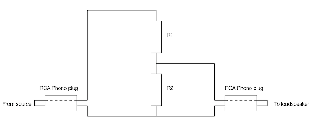
Now we’re going to build a voltage divider. This is device made of two resistors, placed in series (end-to-end) and connected to the output of the source. The point where the two resistors connect together is used as the output to the loudspeaker, resulting in a schematic as shown below.
As you can probably see in the schematic, the grounds of the two devices (which are connected to the exterior casings of the RCA Phono plugs) are connected together. As the voltage on the pin of the source goes up and down, the voltage on the pin of the loudspeaker also goes up and down – but by less. How much less is determined by the values of the resistors.
For example, if the resistors are equal (R1 = R2) then the output will be half of the input. If R2 is one tenth of the total of R1+R2, then the output will be one tenth of the input. You can calculate this gain yourself with a simple equation:
Linear Gain = R2 / (R1 + R2)
and
Gain in dB = 20 * log10 (Linear Gain)
So, for example, if R1 = 8,000 Ω and R2 = 2,000 Ω, then the gain will be
2000 / (8000 + 2000) = 0.2
which is equal to 20*log10 (0.2) -13.98 dB.
Unfortunately, if you want to do this with only two resistors, you can’t be too choosy about their resistances. There are standard resistor values, and you’ll have to pick from that list.
Also, it’s a good “rule of thumb” to try and keep the resistance “seen” by the source around 10,000 Ω (or 10 kΩ) – just to keep it happy. If you make the value too low, then you will be asking for it to deliver too much current (and its maximum output level will drop). If you make it too high, you might create and antenna and result in some extra noise…
So, I want to make R1 +R2 about 10,000 Ω, and I want R2 / (R1+R2) to be about 0.2241 (because I’m trying to convert 29 V RMS to 6.5 V RMS). So, I go to a list of standard resistor values like this one and I start trying to simultaneously fulfill those two requirements.
After some trial and error, I find out that if I make R1 = 8.2 kΩ and R2 = 2.4 kΩ, I can come pretty close.
2400 / (8200 + 2400) = 0.2264 = -12.902
close enough. Now I just need to get a soldering iron and a bit of wire, and put it all together…
The details…
However, if you clicked on that list of standard resistor values, you might notice that it says ±5% at the top of the table. This is normal. If you go to your local resistor store and you buy a 1 kΩ resistor – it probably won’t be exactly 1,000.000000000 Ω. But it will be close. If you buy from the ±5% stack, then any resistor in that bunch will be within 5% of the stated value. So, for a 1 kΩ resistor ±5%, it will be somewhere between 950 Ω and 1050 Ω.
So, then the question is, for the resistors that I just picked, how bad can it get, and is that good enough?
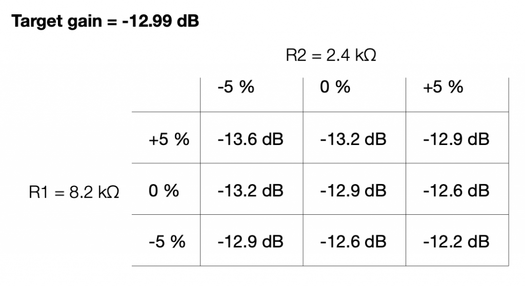
Well… this can be calculated. I just put in the worst-case values for my two resistors into the math, and do it over and over until I get all the possible answers. This would look like this:
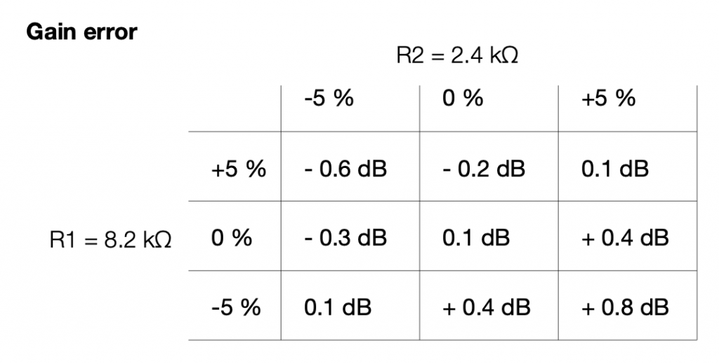
If we look at this in terms of how far away we are from the target – the gain error, then it looks like this:
So, if we randomly choose resistors out of the bag, the worst that can happen is that we will be 0.6 dB below the target or 0.8 dB above the target.
This means that, if we’re not careful, and we’re unlucky, then we can get a mismatch between the two channels of 1.4 dB (assuming that one channel was a worst-case low and the other is a worst-case high). This is enough to be audible as about a 15% shift towards the louder loudspeaker, which is probably not acceptable.
So, the moral of the story is that you should measure your resistors before soldering them into the circuit.
Note, however, that it’s not necessary to make the gains perfect to improve the imaging. You just need to make them equal in the two channels for that…
Speaking Passively
The circuit I show above is called a “passive” circuit. This means that it doesn’t require any external power source (like a battery or a power supply) to work. However, it also means that it can’t make things louder – no matter what resistor values you choose, the output will always be less than the input.
There are lots of reasons why this is a useful little circuit. It’s cheap, it’s easy to make, it’s small (you could hide it inside one of the RCA connectors), and it will prevent you from overloading the input of the downstream device (in this case, a loudspeaker). Not only that, but it will also attenuate the noise generated by the source – so not only will the customer’s system no longer clip, it will also (probably) have a lower noise floor.
Ensemble MidtVest did this recording as part of the commemoration of the 75th anniversary of the Occupation. We recorded the audio in the lobby of Bang & Olufsen’s old headquarters – Gaarden or “The Farm”.
“Love at first sight? Let me just put on my glasses.” Ljupka Cvetanova, The New Land
When I’m working on the sound design for a new pair of (over-ear, closed) headphones, I have to take off my glasses (which makes it difficult for me to see my computer screen…) I’ll explain.
Let’s over-simplify and consider a block diagram of a closed (and therefore “over-ear”) headphone, sitting on one side of your head. This is represented by Figure 1.
Fig 1. A simplified diagram of an over-ear headphone with a sealed cabinet, sitting correctly on the side of your head.
One of the important things to note there is that the air in the chamber between the headphone diaphragm and the ear canal is sealed from the outside world.
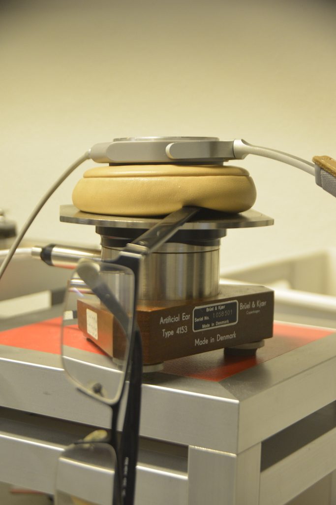
So, if I put such a headphone on an artificial ear (which is a microphone in a small hole in the middle of a plate – it is remarkably well-represented by the red lines in Figure 1….) I can measure its magnitude response. I’ll call this the “reference”. It doesn’t matter to me what the measurement looks like, since this is just a magnitude response which is the combination of the headphone’s response and the artificial ear’s response – with some incorrect positioning thrown into the mix.
Fig 2. The headphones in question, placed on an Artificial Ear for the first measurement.
If I then remove the headphones from the plate, and put them back on, in what I think is the same position, and then do the measurement again, I’ll get another curve.
Then, I’ll subtract the “reference measurement” (the first one) from the second measurement to see what the difference is. An example of this is plotted in Figure 2.
Fig 3. The difference between a magnitude response measurement and the reference measurement of the same ear cup on the same headphones, 1/6th octave smoothed. As you can see, it’s slightly different – but not much. I was VERY careful about re-positioning the headphones on the plate.
Now, let’s consider what happens when the seal is broken. I’ll stick a small piece of metal (actually an Allan key, or a hex wrench, depending on where you live) in between the headphones and the plate, causing a leak in the air between the internal cavity and the outside world, as shown in Figure 4.
Fig 4. A small piece of metal that lifts the leather of the ear cup and causes a small leak around it.
Fig 5. A simplified diagram of an over-ear headphone with a sealed cabinet, sitting incorrectly on the side of your head.
We then repeat the measurement, and subtract the original Reference measurement to see what happened. This is shown in Figure 6.
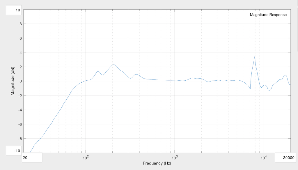
Fig 6. The magnitude response difference caused by a small leak in the chamber.
As you can see, the leak in the system causes us to lose bass, primarily. In the very low end, the loss is significant – more than 10 dB down at 20 Hz! Basically, what we’ve done here is to create an acoustical high-pass filter. (I’m not going to go into the physics of why this happens… That’s too much information for this posting.) You can also see that there’s a bump around 200 Hz which is also a result of the leak. The sharp peak up at 8 kHz is not caused by the leak – it’s just an artefact of the headphones having moved a little on the plate when I put in the Allen Key.
Now let’s make the leak bigger. I’ll stick the arm of my glasses in between the plate and the leather pad.
Fig 7. The arm of my glasses, stuck in the system to make the leak worse…
The result of this measurement (again with the Reference subtracted) is shown in Figure 8.
Fig 8. The magnitude response difference caused by a bigger leak in the chamber.
Now you can see that the high pass filter’s cutoff frequency has risen, and the resonance in the system has not only increased in frequency (to 400 Hz or so) but also in magnitude (to almost +10 dB! Again, the sharp wiggles at the top are mostly just artefacts caused by changes in position…
Just to check and see that I haven’t done something stupid, I’ll remove the glasses, and run the measurement again…
Fig 9. Back to the original – just as a sanity check
The result of this measurement is shown in Figure 10.
Fig 10. Back to a system without leaks… and a magnitude response that closely matches the original – at least in the low end…
So, there are a couple of things to be learned here…
Firstly, if you and a friend both listen to the same pair of closed, sealed headphones, and you disagree about the relative level of bass, check that you’re both not wearing glasses or large earrings…
The more general interpretation of that previous point is that small leaks in the system have a big effect on the response of the headphones in the low-frequency region. Those leaks can happen as a result of many things – not just the arm of your glasses. Hair can also cause the problem. Or, for example, if the headphones are slightly big, and/or your head is slightly small, then the area where your jaw meets your neck under your pinna (around your mastoid gland) is one possile place for leaks. This can also happen if you have a very sharp corner around your jaw (say you are Audrey Hepburn, for example), and the ear cup padding is stiff. Interestingly, as time passes, the foam and covering soften and may change shape slightly to seal these leaks. So, as the headphones match the shape of your head over time, you might get a better seal and a change in the bass level. This might be interpreted by some people as having “broken in” the headphones – but what you’ve actually done is to “break in” the padding so that it fits your head better.
Secondly, those big, sharp spikes up the high end aren’t insignificant… They’re the result of small movements in the headphones on the measuring system. A similar thing happens when you move headphones on your head – but it can be even more significant due to effects caused by your pinna. This is why, many people, when doing headphone measurements, will do many measurements (say, 5 to 10) and average the results. Those errors in placement are not just the result of shifts on the plate – they may also be caused by differences in “clamping pressure” – so, if I angled the headphones a little on that table, then they might be pressing harder on the artificial ear, possibly only on one side of the ear cup, and this will also change the measured response in the high frequency bands.
Fig 11. My glasses on a B&K HATS used for measurements instead of the artificial ear. Check out that leak… This is similar to the problem that I have when I wear glasses when listening to the same headphones.
Of course, it’s possible to reduce this problem by making the foam more compliant (a fancy word for “squishy”) – which may, in turn, mean that the response will be more different for different users due to different head widths. Or the problem could be reduced by increasing the clamping force, which will in turn make the headphones uncomfortable because they’re squeezing your head. Or, you could embrace the leak, and make a pair of open headphones – but those will not give you much passive noise isolation from the outside world. In fact, you won’t have any at all…
So as you can see, as a manufacturer, this issue has to be balanced with other issues when designing the headphones in the first place…
Or you can just take off your glasses, close your eyes, and listen…
Addendum
Please don’t jump too far in your conclusions as a result of seeing these measurements. You should NOT interpret them to mean that, if you wear glasses, you will get a 10 dB bump at 400 Hz. The actual response that you will get from your headphones depends on the size of the leak, the volume of the chamber in the ear cup (which is partly dependent on the size of your pinna, since that occupies a significant portion of the volume inside the chamber) and other factors.
The take-home message here is: when you’re evaluating a pair of closed, over-ear headphones: small leaks have an effect on the low frequency response, and small changes in position have an effect on the high-frequency response. The details of those effects are almost impossible to predict accurately.


