Thanks to George Massenburg at GML Inc. (www.massenburg.com) for his kind
permission to use include this chapter which was originally written as part of a manual
for one of their products.
6.1.1 Introduction
Once upon a time, in the days before audio was digital, when you made a long-distance
phone call, there was an actual physical connection made between the wire
running out of your phone and the phone at the other end. This caused a big
problem in signal quality because a lot of high-frequency components of the signal
would get attenuated along the way. Consequently, booster circuits were made
to help make the relative levels of the various frequencies equal. As a result,
these circuits became known as equalizers. Nowadays, of course, we don’t
need to use equalizers to fix the quality of long-distance phone calls, but we do
use them to customize the relative balance of various frequencies in an audio
signal.
In order to look at equalizers and their smaller cousins, filters, we’re going to have to
look at their frequency response curves. This is a description of how the output level of
the circuit compares to the input for various frequencies. We assume that the input level
is our reference, sitting at 0 dB and the output is compared to this, so if the signal is
louder at the output, we get values greater than 0 dB. If it’s quieter at the output, then we
get negative values at the output.
6.1.2 Filters
Before diving straight in and talking about how equalizers behave, we’ll start
with the basics and look at four different types of filters. Just like a coffee filter
keeps coffee grinds trapped while allowing coffee to flow through, an audio
filter lets some frequencies pass through unaffected while reducing the level of
others.
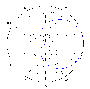
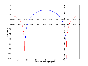
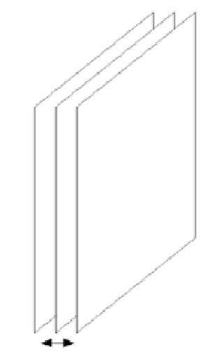
Low-pass Filter
One of the conceptually simplest filters is known as a low-pass filter because it allows
low frequencies to pass through it. The question, of course, is “how low is low?” The
answer lies in a single frequency known as the cutoff frequency or fc. This is the
frequency where the output of the filter is 3.01 dB lower than the maximum output for
any frequency (although we normally round this off to -3 dB which is why it’s usually
called the 3 dB down point). “What’s so special about -3 dB?” I hear you cry. This
particular number is chosen because -3 dB is the level where the signal is at one half the
power of a signal at 0 dB. So, if the filter has no additional gain incorporated into it,
then the cutoff frequency is the one where the output is exactly one half the
power of the input. (Which explains why some people call it the half-power
point.)
As frequencies get higher and higher, they are attenuated more and more. This results
in a slope in the frequency response graph which can be calculated by knowing the
amount of extra attenuation for a given change in frequency. Typically, this slope is
specified in decibels per octave. Since the higher we go, the more we attenuate in a low
pass filter, this value will always be negative.
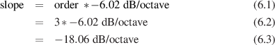
The slope of the filter is determined by its order. If we oversimplify just a little, a
first-order low-pass filter will have a slope of -6.02 dB per octave above its
cutoff frequency (usually rounded to -6 dB/oct). If we want to be technically
correct about this, then we have to be a little more specific about where we
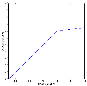
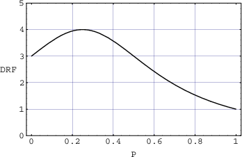
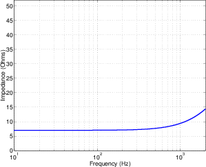
finally reach this slope. Take a look at the frequency response plot in Figure
6.1. Notice that the graph has a nice gradual transition from a slope of 0 (a
horizontal line) in the really low frequencies to a slope of -6 dB/oct in the really
high frequencies. In the area around the cutoff frequency, however, the slope is
changing. If we want to be really accurate, then we have to say that the slope of
the frequency response is really 0 for frequencies less than one tenth of the
cutoff frequency. In other words, for frequencies more than one decade below
the cutoff frequency. Similarly, the slope of the frequency response is really
-6.02 dB/oct for frequencies more than one decade above (ten times) the cutoff
frequency.
If we have a higher-order filter, the cutoff frequency is still the one where the output
drops by 3 dB, however the slope changes to a value of -6.02n dB/oct, where n is the
order of the filter. For example, if you have a 3rd-order filter, then the slope
is
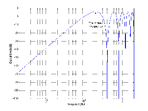
High-pass Filter
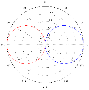
A high-pass filter is essentially exactly the same as a low-pass filter, however, it permits
high frequencies to pass through while attenuating low frequencies as can be seen in
Figure 6.2. Just like in the previous section, the cutoff frequency is where the
output has a level of -3.01 dB but now the slope below the cutoff frequency is
positive because we get louder as we increase in frequency. Just like the low-pass
filter, the slope of the high-pass filter is dependent on the order of the filter and
can be calculated using the equation 6.02n dB/oct, where n is the order of the
filter.
Remember as well that the slope only applies to frequencies that are at least one
decade away from the cutoff frequency.
Band-pass Filter
Let’s take a signal and send it through a high-pass filter and a low-pass filter in series, so
the output of one feeds into the input of the other. Let’s also assume for a moment that
the two cutoff frequencies are more than a decade apart.
The result of this probably won’t hold any surprises. The high-pass filter will
attenuate the low frequencies, allowing the higher frequencies to pass through. The
low-pass filter will attenuate the high frequencies, allowing the lower frequencies to pass
through. The result is that the high and low frequencies are attenuated, with a middle
band (called the passband) that’s allowed to pass relatively unaffected.
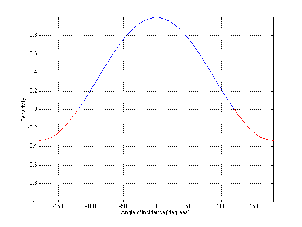
Bandwidth
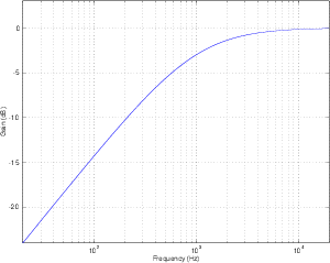
The system described in the previous section is called a bandpass filter and it has a
couple of specifications that we should have a look at. The first is the width of the
passband. This bandwidth is calculated using the difference two cutoff frequencies which
we’ll label fc1 for the lower one and fc2 for the higher one. Consequently, the bandwidth
is calculated using the equation:
 | (6.4) |
So, using the example of the filter frequency response shown in Figure 6.3, the
bandwidth is 5,000 Hz – 100 Hz = 4900 Hz.
Centre Frequency
We can also calculate the middle of the passband using these two frequencies. It’s not
quite so simple as we’d like, however. Unfortunately, it’s not just the frequency
that’s half-way between the low and high frequency cutoff’s. This is because
frequency specifications don’t really correspond to the way we hear things.
Humans don’t usually talk about frequency – they talk about pitches and notes.
They say things like “Middle C” instead of “262 Hz.” They also say things
like “one octave” or “one semitone” instead of things like “a bandwidth of 262
Hz.”
Consider that, if we play the A below Middle C on a well-tuned piano, we’ll hear a
note with a fundamental of 220 Hz. The octave above that is 440 Hz and the octave above
that is 880 Hz. This means that the bandwidth of the first of these two octaves is 220
Hz (it’s 440 Hz – 220 Hz), but the bandwidth of the second octave is 440 Hz
(880 Hz – 440 Hz). Despite the fact that they have different bandwidths, we
hear them each as one octave, and we hear the 440 Hz note as being half-way
between the other two notes. So, how do we calculate this? We have to find what’s
known as the geometric mean of the two frequencies. This can be found using the
equation
Q
Let’s say that you want to build a bandpass filter with a bandwidth of one octave. This
isn’t difficult if you know the centre frequency and if it’s never going to change. For
example, if the centre frequency was 440 Hz, and the bandwidth was one octave wide,
then the cutoff frequencies would be 311 Hz and 622 Hz (we won’t worry too much at
the moment about how I arrived at these particular numbers). What happens if we
leave the bandwidth the same at 311 Hz, but change the centre frequency to
880 Hz? The result is that the bandwidth is now no longer an octave wide –
it’s one half of an octave. So, we have to link the bandwidth with the centre
frequency so that we can describe it in terms of a fixed musical interval (for you
engineers, a musical interval is a measure of the distance between two notes). This is
done using what is known as the quality or Q of the filter, calculated using the
equation:
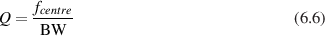
Now, instead of talking about the bandwidth of the filter, we can use the Q which
gives us an idea of the width of the filter in musical terms. This is because, as we increase
the centre frequency, we have to increase the bandwidth proportionately to maintain the
same Q. Notice however, that if we maintain a centre frequency, the smaller the
bandwidth gets, the bigger the Q becomes, so if you’re used to talking in terms of
musical intervals, you have to think backwards. The bigger the Q, the smaller the
interval.
Remember that you can have a very high Q, and therefore a very narrow
bandwidth for a bandpass filter. All of the definitions still hold, however. The cutoff
frequencies are still the points where we’re 3 dB lower than the maximum value and
the bandwidth is still the distance in Hertz between these two points and so
on...
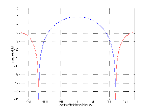
Band-reject Filter
Although bandpass filters are very useful at accentuating a small band of frequencies
while attenuating others, sometimes we want to do the opposite. What if we want to
attenuate a small band of frequencies while leaving the rest alone? This can be
accomplished using a band-reject filter (also known as a bandstop filter) which, as its
name implies, rejects (or usually just attenuates) a band of frequencies without affecting
the surrounding material. The frequency response of this can be seen in Figure
6.4.
The thing to be careful of when describing band-reject filters is the fact that cutoff
frequencies are still defined as the points where we’ve dropped in level by 3 dB from the
maximum output.
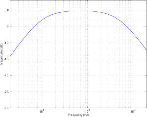
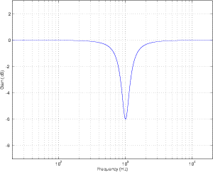
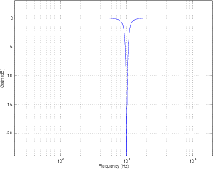
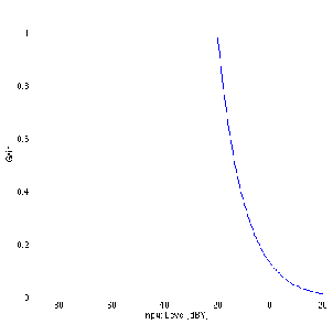
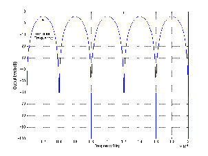
Notch Filter
There is a special breed of band-reject filter that is designed to have almost infinite
attenuation at a single frequency, leaving all others intact. This, of course is impossible,
but we can come close. If we have a band-reject filter with a very high Q, the result is a
frequency response like the one shown in Figure 6.5. The shape is basically a flat
frequency response with a narrow, deep notch at one frequency – hence the name notch
filter
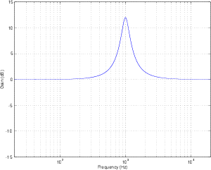
Peak Filter
There is a variation on the bandpass filter that, instead of attenuating all frequencies
outside the passband, the filter typically leaves them at a gain of 0 dB. This kind of filter
can be seen in the plot of an in Figure 6.6 and is called a peaking filter or peak filter.
Notice now that, rather than attenuating all unwanted frequencies, the filter can be
thought of as simply applying a known gain in the passband. The further away you get
from the passband, the less the signal is affected. Notice, however, that we still measure
the bandwidth using the two points that are 3 dB down from the peak of the
curve.
In most instances of these kinds of filters, it is also possible to attenuate the same
frequency band, as is shown in Figure 6.10. Since the practical implementation of this
filter allows you to boost and attenuate, they are commonly known of as peak/dip
filters.
6.1.3 Equalizers
Unlike its counterpart from the days of long-distance phone calls, a modern
equalizer is a device that is capable of attenuating and boosting frequencies
according to the desire and expertise of the user. There are four basic types of
equalizers, but we’ll have to talk about a couple of issues before getting into the
nitty-gritty.
An equalizer typically consists of a collection of filters, each of which permits you to
control one or more of three things: the gain, centre frequency and Q of the filter. There
are some minor differences in these filters from the ones we discussed above, but
we’ll sort that out before moving on. Also, the filters in the equalizer may be
connected in parallel or in series, depending on the type of equalizer and the
manufacturer.
To begin with, as we’ll see, a filter in an equalizer comes in two basic models, the
peak/dip filter and the shelving filter which is a type of variation on the highpass and low
pass filters.
Filter symmetry
Constant Q Filter
Let’s look at the frequency response of a filter with a centre frequency of 1 kHz, a Q of 4
and a two different amounts of boost or cut. If we plot these responses on the same
graph, they look like Figure 6.11.
Notice that, although these two curves have “matching” parameters, they do not have
the same shape. This is because the bandwidth (and therefore the Q) of a filter is
measured using its 3 dB down point – not the point that’s 3 dB away from the peak or
dip in the curve. Since the measurement is not symmetrical, the curves are not
symmetrical. This is true of any filter where the Q is kept constant and gain is modified.
If you compare a boost of any amount with a cut of the same amount, you’ll
always get two different curves. This is what is known as a constant Q filter
because the Q is kept as a constant. The result is called an asymmetrical filter (or
non-symmetrical filter) because a matching boost and cut are not mirror images of each
other.
There are advantages and disadvantages to this type of filter. The primary advantage
is that you can have a very selective cut if you’re trying to eliminate a single
frequency, simply by increasing the Q. The primary disadvantage is that you cannot
undo what you have done. This last statement is explained in the following
section.
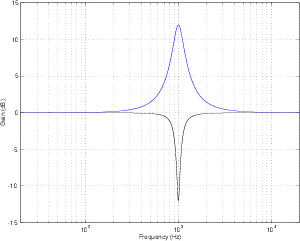
Reciprocal Peak/Dip Filter
Instead of building a filter where the cut and boost always maintain a constant Q, let’s set
about to build a filter that is symmetrical – that is to say that a matching boost and cut at
the same centre frequency would result in the same shape. The nice thing about this
design is that, if you take two such filters and connect them in series and set their
parameters to be the same but opposite gains (for example, both with a centre frequency
of 1 kHz and a Q of 2, but one has a boost of 6 dB and the other has a cut of 6 dB) then
they’ll cancel each other out and your output will be identical to your input. This also
applies if you’ve equalized something while recording – assuming that you live in
a perfect world, if you remember your original settings on the recorded EQ
curve, you can undo what you’ve done by duplicating the settings and inverting
the gain. As a result, we call this a reciprocal peak/dip filterfilter, reciprocal
peak/dip.
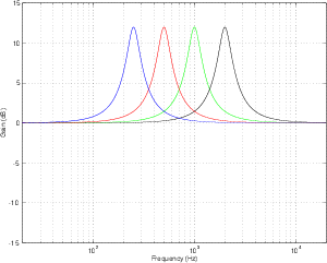
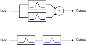
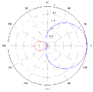
Parallel vs. Series Filters
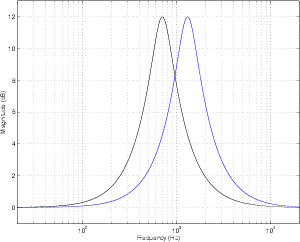
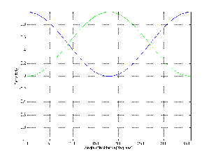
Let’s take two reciprocal peak/dip filters, each set with a Q of 2 and a gain of 6 dB. The
only difference between them is that one has a centre frequency of 700 Hz and the other
has a centre frequency of 1.3 kHz. If we use both of these filters on the same signal
simultaneously, we can achieve two very different resulting frequency responses,
depending on how they’re connected.
If the two filters are connected in series (it doesn’t matter what order we connect
them in), then the frequency band that overlaps in the boosted portion of the two filters’
responses will be boosted twice. In other words, the signal goes through the first filter
and is amplified, after which it goes through the second filter and the amplified signal is
boosted further. This arrangement is also known as a circuit made of combining
filters.
If we connect the two filters in parallel, however, a different situation occurs. Now
each filter boosts the original signal independently, and the two resulting signals are
added, producing a small increase in level, but not as significant as in the case of the
series connection. This arrangement is also known as a circuit made of non-combining
filters.
The primary advantage to having filters in connected in series rather than in parallel
lies in possibility of increased gain or attenuation. For example, if you have two
filters in series, each with a boost of 12 dB and with matched centre frequencies,
the total resulting gain applied to the signal is 24 dB (because a gain of 12 dB
from the second filter is applied to a signal that already has a gain of 12 dB
from the first filter). If the same two filters were connected in parallel, the total
maximum gain would be only 18 dB. (This is because a the addition of two identical
signals results in a doubling of level which corresponds to an additional gain
of only 6 dB. Note as well that the overall gain of a parallel connection is 6
dB.)
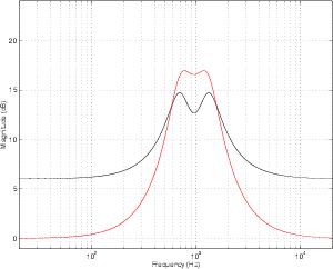
The main disadvantage to having filters connected in series rather than in
parallel is the fact that you can occasionally result in frequency bands being
boosted more than you’re intuitively aware. For example, looking at Figure 6.16,
we can see that, based on the centre frequencies of the two filters, we would
expect to have two narrow peaks in the total frequency response at 700 Hz and
1.3 kHz. The actual result, as can be seen, is a (sort of...) single broad peak
between the two expected centre frequencies. Also, it should be noted that a
group of non-combining filters will likely a ripple in their output frequency
response.
Shelving Filter
The nice thing about high pass and low pass filters is that you can reduce (or eliminate)
things you don’t want (like low-frequency noise from air conditioners, for example.) But,
what if you want to boost all your low frequencies instead of cutting all your
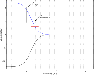
high’s? This is when a shelving filter comes in handy. The response curve of
shelving filters most closely resemble their high- and low-pass filter counterparts
with a minor difference. As their name suggests, the curve of these filters level
out at a specified frequency called the stop frequency. In addition, there is a
second defining frequency called the turnover frequency which is the frequency at
which the response is 3 dB above or below 0 dB. This is illustrated in Figure
6.17.
The transition ratio is sort of analogous to the order of the filter and is calculated
using the turnover and stop frequencies as shown below.
where RT is the transition ratio.
The closer the transition ratio is to 1, the greater the slope of the transition in gain
from the unaffected to the affected frequency ranges. This is because if RT = 1 then
fstop = fturnover.
These filters are available as high- and low-frequency shelving units, boosting high
and low frequencies respectively. In addition, they typically have a symmetrical
response. If the transition ratio is less than 1, then the filter is a low shelving
filter. If the transition ratio is greater than 1, then the filter is a high shelving
filter.
The disadvantage of these components lies in their potential to boost frequencies
above and below the audible audio range causing at the least wasted amplifier power and
at the worst, loudspeaker damage. For example, if you use a high shelf filter with a stop
frequency of 10 kHz to increase the level of the high end by 12 dB to brighten things up a
bit, you will probably also wind up boosting signals above your hearing range. In a
typical case, this may cause some unpredictable signals from your tweeter due to
increased intermodulation distortion of signals you can’t even hear. To reduce these
unwanted effects, super sonic and subsonic signals can be attenuated using a low pass or
high pass filter respectively outside the audio band. Using a peaking filter at the
appropriate frequency instead of a filter with a shelving response can avoid the problem
altogether.
The most common application of this equalizer is the tone controls on home sound
systems. These bass and treble controls generally have a maximum slope of 6 dB per
octave and reciprocal characteristics. They are also frequently seen on equalizer modules
on small mixing consoles.
Graphic Equalizer
Graphic equalizers are seen just about everywhere these days, primarily because they’re
intuitive to use. In fact, they are probably the most-used piece of signal processing
equipment in recording. The name “graphic equalizer” comes from the fact that the
device is made up of a number of filters with centre frequencies that are regularly spaced,
each with a slider used for gain control. The result is that the arrangement of the sliders
gives a graphic representation of the frequency response of the equalizer. The most
common frequency resolutions available are one-octave, two-third-octave and
one-third-octave, although resolutions as fine as one-twelveth-octave exist. The sliders on
most graphic equalizers use ISO standardized band center frequencies (See
Section 12.1). They almost always employ reciprocal peak/dip filters wired
in parallel. As a result, when two adjacent bands are boosted, there remains
a comparatively large dip between the two peaks. This proves to be a great
disadvantage when attempting to boost a frequency between two center frequencies.
Drastically excessive amounts of boost may be required at the band centers in
order to properly adjust the desired frequency. This problem is eliminated in
graphic EQ’s using the much-less-common combining filters. In this system, the
filter banks are wired in series, thus adjacent bands have a cumulative effect.
Consequently, in order to boost a frequency between two center frequencies, the given
filters need only be boosted a minimal amount to result in a higher-boosted
mid-frequency.
Virtually all graphic equalizers have fixed frequencies and a fixed Q. This
makes them simple to use and quick to adjust, however they are generally a
compromise. Although quite suitable for general purposes, in situations where a
specific frequency or bandwidth adjustment is required, they will prove to be
inaccurate.
Paragraphic Equalizer
One attempt to overcome the limitations of the graphic equalizer is the paragraphic
equalizer. This is a graphic equalizer with fine frequency adjustment on each
slider. This gives the user the ability to sweep the center frequency of each
filter somewhat, thus giving greater control over the frequency response of the
system.
Sweep Filters
These equalizers are most commonly found on the input stages of mixing consoles. They
are generally used where more control is required over the signal than is available with
graphic equalizers, yet space limitations restrict the sheer number of potentiometers
available. Typically, the equalizer section on a console input strip will have one or
two sweep filters in addition to low and a high shelf filters with fixed turnover
frequencies. The frequencies of the mid-range filters are usually reciprocal
peak/dip filters with an adjustable (or sweepable) center frequencies and fixed
Q’s.
The advantage of this configuration is a relatively versatile equalizer with a minimum
of knobs, precisely what is needed on an overcrowded mixer panel. The obvious
disadvantage is its lack of adjustment on the bandwidth, a problem that is solved with a
parametric equalizer.
Parametric Equalizer
A parametric equalizer is one that allow the user to control the gain, centre frequency
and Q of each filter. In addition, these three parameters are independent – that is to say
that adjusting one of the parameters will have no effect on the other two. They are
typically comprised of combining filters and will have either reciprocal peak/dip or
constant-Q filters. (Check your manual to see which you have – it makes a huge
difference!) In order to give the user a wider amount of control over the signal, the
frequency ranges of the filters in a parametric equalizer typically overlap, making it
possible to apply gain or attenuation to the same centre frequency using at least two
filters.
The obvious advantage of using a parametric equalizer lies in the detail and
versatility of control afforded by the user. This comes at a price, however – it
unfortunately takes much time and practice to master the use of a parametric
equalizer.
Semi-parametric equalizer
A less expensive variation on the true parametric equalizer is the semi-parametric
equalizer or quasi-parametric equalizer. From the front panel, this device appears to be
identical to its bigger cousin, however, there is a significant difference between the two.
Whereas in a true parametric equalizer, the three parameters are independent, in a
semi-parametric equalizer, they are not. As a result, changing the value of one
parameter will cause at least one, if not both, of the other two parameters to change
unexpectedly. As a result, although these devices are less expensive than a true
parametric, they are less trustworthy and therefore less functional in real working
situations.
|
|
|
|
|
|
| Category | Graphic | | Parametric
|
|
|
|
|
|
|
| Control | Graphic | Paragraphic | Sweep | Semi-parametric | True Parametric |
| Gain | Y | Y | Y | Y | Y |
| Centre Frequency | N | Y | Y | Y | Y |
| Q | N | N | N | Y | Y |
| Shelving Filter? | N | N | Y | Optional | Optional |
| Combining / Non-combining | N | N | N | Depends | C |
| Reciprocal peak/dip or Constant Q | R p/d | R p/d | R p/d | Typically R p/d | Depends |
|
|
|
|
|
|
| |
Table 6.1: Summary of the typical control characteristics on the various types of
equalizers. “Depends” means that it depends on the manufacturer and model.
6.1.4 Phase response
So far, we’ve only been looking at the frequency response of a filter or equalizer. In other
words, we’ve been looking at what the magnitude of the output of the filter would be if
we send sine tones through it. If the filter has a gain of 6 dB at a certain frequency,
then if we feed it a sine tone at that frequency, then the amplitude of the output
will be 2 times the amplitude of the input (because a gain of 2 is the same as
an increase of 6 dB). What we haven’t looked at so far is any shift in phase
(also known as phase distortion) that might be incurred by the filtering process.
Any time there is a change in the frequency response in the signal, then there
is an associated change in phase response that you may or may not want to
worry about. That phase response is typically expressed as a shift (in degrees)
for a given frequency. Positive phase shifts mean that the signal is delayed in
phase whereas negative phase shifts indicate that the output is ahead of the
input.
“The output is ahead of the input!?” I hear you cry. “How can the output be ahead of
the input? Unless you’ve got one of those new digital filters that can see into the near
future...” Well, it’s actually not as strange as it sounds. The thing to remember here is that
we’re talking about a sine wave – so don’t think about using an equalizer to help your
drummer get ahead of the beat... It doesn’t mean that the whole signal comes out earlier
than it went in. This is because we’re not talking about negative delay – it’s negative
phase.
Minimum phase
While it’s true that a change in frequency response of a signal necessarily implies that
there is a change in its phase, you don’t have to have the same phase shift for the same
frequency response change. In fact, different manufacturers can build two filters with
centre frequencies of 1 kHz, gains of 12 dB and Q’s of 4. Although the frequency
responses of the two filters will be identical, their phase responses can be very
different.
You may occasionally hear the term minimum phase to describe a filter. This is a
filter that has the frequency response that you want, and incurs the smallest (hence
“minimum”) shift in phase to achieve that frequency response.
Two things to remember about minimum phase filters: 1) Just because they have the
minimum possible phase shift doesn’t necessarily imply that they sound the best. 2) A
minimum phase filter can be “undone” – that is to say that if you put your signal through
a minimum phase filter, it is possible to find a second minimum phase filter that
will reverse all the effects of the first, giving you exactly the signal you started
with.
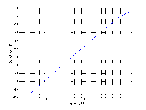
Linear phase
If you plot the phase response of a filter for all frequencies, chances are you’ll get a
smooth, fancy-looking curve like the ones in Figure 6.18. Some filters, on the other hand,
have a phase response plot that’s a straight line if you graph the response on a
linear frequency scale (instead of a log scale like we normally do...). This line
usually slopes upwards so the higher the frequency, the bigger the phase change.
In fact, this would be exactly the phase response of a straight delay line – the
higher the frequency, the more of a phase shift that’s incurred by a fixed delay
time. If the delay time is 0, then the straight line is a horizontal one at 0∘ for all
frequencies.
Any filter whose phase response is a straight line is called a linear phase filter. Be
careful not to jump to the conclusion that, because it’s a linear phase filter, it’s better than
anything else. While there are situations where such a filter is useful, they don’t
necessarily work well in all situations to correct all problems. Different intentions require
different filter characteristics.
Ringing
The phase response of a filter is typically strongly related to its Q. The higher the Q (and
therefore the smaller the bandwidth) the greater the change in phase around the
centre frequency. This can be seen in Figure 6.18 above. Notice that, the higher
the Q, the higher the slope of the phase response at the centre frequency of
the filter. When the slope of the phase response of a filter gets very steep (in
other words, when the Q of the filter is very high) an interesting thing called
ringing happens. This is an effect where the filter starts to oscillate at its centre
frequency for a length of time after the input signal stops. The higher the Q, the
longer the filter will ring, and therefore the more audible the effect will be. In
the extreme cases, if the Q of the filter is 0, then there is no ringing (but the
bandwidth is infinity and you have a flat frequency response – so it’s not a very
useful filter...). If the Q of the filter is infinity, then the filter becomes a sine wave
generator.
6.1.5 Applications
All this information is great – but why and how would you use an equalizer?
Spectral sculpting
This is probably the most obvious use for an equalizer. You have a lead vocal that
sounds too bright so you want to cut back the high frequency content. Or you
want to bump up the low mid range of a piano to warm it up a bit. This is the
primary intention of the tone controls on the cheapest ghetto blaster through to
the best equalizer in the recording studio. It’s virtually impossible to give a
list of “tips and tricks” in this category, because every instrument and every
microphone in every recording situation will be different. There are time when
you’ll want to use an equalizer to compensate for deficiencies in the signal
because you couldn’t afford a better mic for that particular gig. On the other
hand there may be occasions where you have the most expensive microphone in
the world on a particular instrument and it still needs a little tweaking to fix it
up. There are, however, a couple of good rules to follow when you’re in this
game.
First of all – don’t forget that you can use an equalizer to cut as well as
boost. Consider a situation where you have a signal that has too much bass
– there are two possible ways to correct the problem. You could increase the
mids and highs to balance, or you could turn down the bass. There are as many
situations where one of these is the correct answer as there are situations where
the other answer is more appropriate. Try both unless you’re in a really big
hurry.
Second of all – don’t touch the equalizer before you’ve heard what you’re tweaking. I
often notice when I go to a restaurant that there are a huge number of people who put salt
and pepper on their meal before they’ve even tasted a single morsel. Doesn’t make much
sense... Hand them a plate full of salt and they’ll still shake salt on it before raising a
hand to touch their fork. The same goes for equalization. Equalize to fix a problem that
you can hear – not because you found a great EQ curve that worked great on kick drum
at the last session.
Thirdly – don’t overdo it. Or at least, overdo it to see how it sounds when it’s
overdone, then bring it back. Again, back to a restaurant analogy – you know that
you’re in a restaurant that knows how to cook steak when there’s a disclaimer
on the menu that says something to the effect of “We are not responsible for
steaks ordered well done.” Everything in moderation – unless, of course, you’re
intending to plow straight through the fields of moderation and into the barn of
excess.
Fourthly, there’s a number of general descriptions that indicate problems that can be
fixed, or at least tamed with equalization. For example, when someone says that the
sound is “muddy,” you could probably clean this up by reducing the area around 125 –
250 Hz with a low-Q filter. Table 6.2 gives a number of basic examples, but there are
plenty more – ask around...
|
|
| Symptom description | Possible remedy |
|
|
| Bright | Reduce high frequency shelf |
| Dark, veiled, covered | Increase high frequency shelf |
| Harsh, crunchy | Reduce 3 – 5 kHz region |
| Muddy, thick | Reduce 125 – 250 Hz region |
| Lacks body or warmth | Increase 250 – 500 Hz |
| Hollow | Reduce 500 Hz region |
|
|
| |
Table 6.2: Some possible spectral solutions to general comments about the sound
quality
One last trick here applies when you hear a resonant frequency sticking out, and you
want to get rid of it, but you just don’t know what the exact frequency is. You know that
you need to use a filter to reduce a frequency – but finding it is going to be
the problem. The trick is to search and destroy by making the problem worse.
Set a filter to boost instead of cutting a frequency band with a fairly high Q.
Then, sweep the frequency of the filter until the resonance sticks out more than
it normally does. You can then fine tune the centre frequency of the filter so
that the problem is as bad as you can make it, then turn the boost back to a
cut.
Loudness
Although we rarely like to admit it, we humans aren’t perfect. This is true in many
respects, but for the purposes of this discussion, we’ll concentrate specifically on our
abilities to hear things. Unfortunately, our ears don’t have the same frequency response at
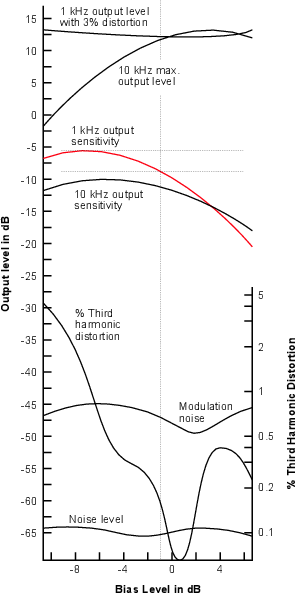
all listening levels. At very high listening levels, we have a relatively flat frequency
response, but as the level drops, so does our sensitivity to high and low frequencies. (This
effect was discussed in Section 5.4.) As a result, if you mix a tune at a very high listening
level and then reduce the level, it will appear to lack low end and high end. Similarly, if
you mix at a low level and turn it up, you’ll tend to hear more low end and high
end.
One possible use for an equalizer is to compensate for the perceived lack of
information in extreme frequency ranges at low listening levels. Essentially, when you
turn down the monitor levels, you can use an equalizer to increase the levels of the low
and high frequency content to compensate for deficiencies in the human hearing
mechanism. This filtering is identical to that which is engaged when you press the
“loudness” button on most home stereo systems. Of course, the danger with such
equalization is that you don’t know what frequency ranges to alter, and how much to
alter them – so it is not recommendable to do such compensation when you’re
mixing, only when you’re at home listening to something that’s already been
mixed.
Noise Reduction
It’s possible in some specific cases to use equalization to reduce noise in recordings, but
you have to be aware of the damage that you’re inflicting on some other parts of the
signal.
High-frequency Noise (Hiss)
Let’s say that you’ve got a recording of an electric bass on a really noisy analog tape
deck. Since most of the perceivable noise is going to be high-frequency stuff and since
most of the signal that you’re interested in is going to be low-frequency stuff, all you
need to do is to roll off the high end to reduce the noise. Of course, this is be best of all
possible worlds. It’s more likely that you’re going to be coping with a signal that has
some high-frequency content (like your lead vocals, for example...) so if you start rolling
off the high end too much, you start losing a lot of brightness and sparkle from your
signal, possibly making the end result worse that you started. If you’re using equalization
to reduce noise levels, don’t forget to occasionally hit the “bypass” switch of the
equalizer once and a while to hear the original. You may find when you refresh
your memory that you’ve gone a little too far in your attempts to make things
better.
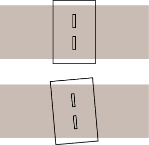
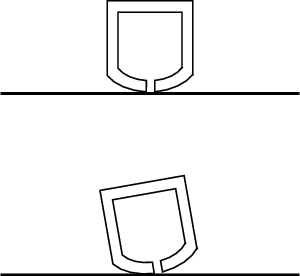
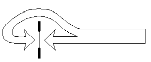
Low-frequency Noise (Rumble)
Almost every console in the world has a little button on every input strip that
has a symbol that looks like a little ramp with the slope on the left. This is a
high-pass filter that is typically a second-order filter with a cutoff frequency
around 100 Hz or so, depending on the manufacturer and the year it was built.
The reason that filter is there is to help the recording or sound reinforcement
engineer get rid of low-frequency noise like “stage rumble” or microphone
handling noise. In actual fact, this filter won’t eliminate all of your problems,
but it will certainly reduce them. Remember that most signals don’t go below
100 Hz (this is about an octave and a half below middle C on a piano) so you
probably don’t need everything that comes from the microphone in this frequency
range – in fact, chances are, unless you’re recording pipe organ, electric bass or
space shuttle launches, you won’t need nearly as much as you think below 100
Hz.
Hummmmmmm...
There are many reasons, forgivable and unforgivable, why you may wind up with an
unwanted hum in your recording. Perhaps you work with a poorly-installed system.
Perhaps your recording took place under a buzzing streetlamp. Whatever the reason, you
get a single frequency (and perhaps a number of its harmonics) singing all the way
through your recording. The nice thing about this situation is that, most of the
time, the hum is at a predictable frequency (depending on where you live, it’s
likely a multiple of either 50 Hz or 60 Hz) and that frequency never changes.
Therefore, in order to reduce, or even eliminate this hum, you need a very narrow
band-reject filter with a lot of attenuation. Just the sort of job for a notch filter. The
drawback is that you also attenuate any of the music that happens to be at or
very near the notch centre frequency, so you may have to reach a compromise
between eliminating the hum and having too detrimental of an effect on your
signal.
Dynamic Equalization
A dynamic equalizer is one which automatically changes its frequency response
according to characteristics of the signal passing through it. You won’t find many single
devices what fit this description, but you can create a system that behaves differently for
different input signals if you add a compressor to the rack. This is easily accomplished
today with digital multi-band compressors which have multiple compressors
fed by what could be considered a crossover network similar to that used in
loudspeakers.
Dynamic enhancement
Take your signal and, using filters, divide it into two bands with a crossover
frequency at around 5 kHz. Compress the higher band using a fast attack and release
time, and adjust the output level of the compressor so that when the signal is at a peak
level, the output of the compressor summed with the lower frequency band results in a
flat frequency response. When the signal level drops, the low frequency band will be
reduced more than the high frequency band and a form of high-frequency enhancement
will result.
Dynamic Presence
In order to add a sensation of “presence” to the signal, use the technique described in
Section 6.1.5 but compress the frequency band in the 2 kHz to 5 kHz range instead of all
high frequencies.
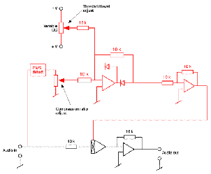
De-Essing
There are many instances where a close-mic technique is used to record a narrator
and the result is a signal that emphasizes the sibilant material in the signal – in particular
the “s” sound. Since the problem is due to an excess of high frequency, one option to fix
the issue could be to simply roll off high frequency content using a low-pass filter or a
high-frequency shelf. However, this will have the effect of dulling all other
material in the speech, removing not only the “s’s” but all brightness in the signal.
The goal, therefore, is to reduce the gain of the signal when the letter “s” is
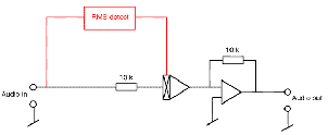
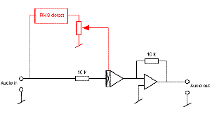
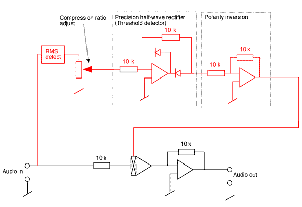
spoken. This can be accomplished using an equalizer and a compressor with a
side chain. In this case, the input signal is routed to the inputs of the equalizer
and the compressor in parallel. The equalizer is set to boost high frequencies
(thus making the “s’s” even louder...) and its output is fed to the side chain
input of the compressor. The compression parameters are then set so that the
signal is not normally compressed, however, when the “s” is spoken, the higher
output level from the equalizer in the side chain triggers compression on the
signal. The output of the compressor has therefore been “de-essed” or reduced in
sibilance.
Although it seems counterintuitive, don’t forget that, in order to reduce
the level of the high frequencies in the output of the compressor, you have to
increase the level of the high frequencies at the output of the equalizer in this
case.
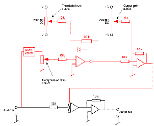
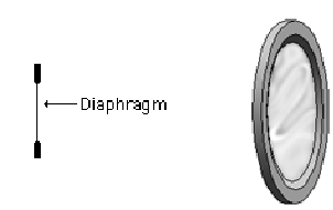
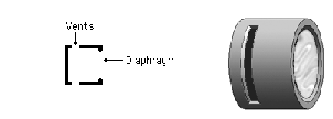
Pop-reduction
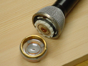
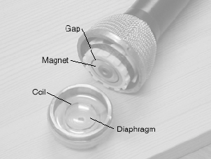
A similar problem to de-essing is the “pop” that occurs when a singer’s plosive
sounds (p’s and b’s) cause a thump at the diaphragm of the microphone. There is a
resulting overload in the low frequency component of the signal that can be eliminated
using the same technique described in Section 6.1.5 where the low frequencies
(250 Hz and below) are boosted in the equalizer instead of the high frequency
components.
6.1.6 Beware! Q is not constant!
We saw above that the quality factor, or Q, is defined by the centre frequency and the
bandwidth of the filter. That bandwidth is defined using the two cutoff frequencies of the
filter’s response, which are, in turn, defined using a -3 dB point. So, to find the cutoff
frequencies, you find the peak in the filter’s response, and then go 3 dB below that and
find the frequencies that intersect that level.
However, this results in some strange effects as we saw above. If you have a peaking
filter, then your cutoff frequencies are 3 dB below the peak – the maximum
effect in your gain. However, if you have a notch filter, then your -3 dB point is
measured down from the part of the response that is unaffected. This is why a
constant-Q peak/dip filter is asymmetrical. If you want to make a reciprocal peak/dip
filter, you have to change your definition a little so that, if you’re applying a
dip, then you measure the bandwidth using the points that at 3 dB up from the
bottom of the dip, so we’re not really following the definition of bandwidth (or Q)
properly.
Another problem arises when you have a peak gain that is less than 3 dB. Let’s say
that you use a reciprocal peak/dip filter to apply a gain of 2 dB. This means that no point
in the response is 3 dB lower than the peak, so it therefore has no definable bandwidth or
Q? Hmmmmm.....
There have been some suggested solutions to these problems that have become
commonplace in the gear that we use every day. As a result, if you’re really picky about
what you’re doing, you should be aware of the variations on Q.
Constant Q
As we saw above, if the Q and bandwidth are always defined by the -3 dB point, then you
result in a constant Q behaviour in a peak/dip filter, and therefore an asymmetrical
behaviour.
3 dB down / 3 dB up modification
The simplest solution to this problem of asymmetry is to re-define bandwidth when you
have a dip – therefore using the 3 dB up points instead.
However, both this method, and the Constant Q method suffer from the problem of
what the bandwidth and Q are when the gain is greater than -3 dB and less than 3 dB
(since you can’t find a point in a magnitude response that’s 3 dB down when the highest
peak is less than 3 dB up...).
Half-gain defined Q – Hybrid
One solution that was offered [Moorer, 1983] to get around the problem of gains below 6
dB was to re-define the bandwidth so that, whenever the peak gain is less than 6 dB, you
use the gain value that is half of the peak value. For example, if the gain is 6 dB, then you
define your bandwidth using the point 3 dB down from that (half of 6 is 3). If the gain is
4 dB, then you define bandwidth using the 2 dB-down (relative to the peak)
point.
The nice thing about this definition is that, by using half of the gain to define the
bandwidth (and therefore the Q) you automatically get a reciprocal (and therefore
symmetrical) shape for peaks and dips.
Half-gain defined Q
Finally, along came a guy named Robert Bristow-Johnson who suggested that, since
using the half-gain point to define Q was so useful (particularly in making reciprocal
filters) then we should use it all the time[Bristow-Johnson, 1994].
There are two catches here. The first is that he suggested that we use this new
definition not only for peak/dip filters, but shelving filters as well. The second is that he
put a set of equations on Usenet (a precursor to the World Wide Web - where they live
today at http://www.musicdsp.org/files/Audio-EQ-Cookbook.txt) that are used to
implement the filters. Since those equations were freely available, everyone (well, almost
everyone) uses them when they’re building the equalisers that you use in the gear that
you buy.
How different are they?
Well... the big question here is whether or not you care that these differences exist.
Maybe not. Personally, I do... however, it’s for a very good reason. If I implement an EQ
curve on one piece of gear and write down my parameters (type, centre or cutoff
frequency, gain and Q) I expect to be able to put those parameters in another piece of
gear and get exactly the same response out. This won’t happen if the people who made
your equalisers use different definitions of Q. This might be very bad... How bad? Well,
let’s take a look...
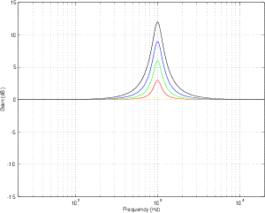
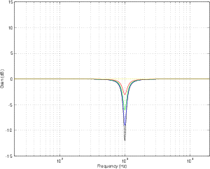
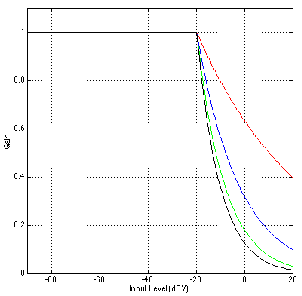
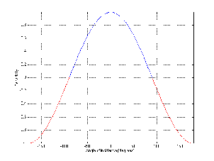
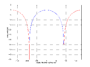
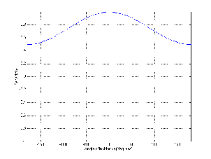
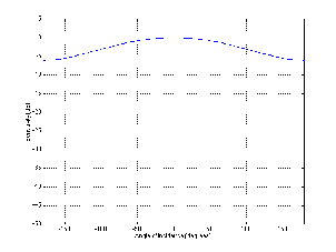
Changes in gain
Figures 6.21 and 6.22 shows the difference in gain and phase respectively between
two filters, both with an fc of 1 kHz and a Q of 2 and three different gains. However, one
filter calculates Q based on the 3 dB down point, the other based on the midpoint of the
maximum gain.
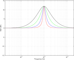
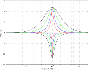
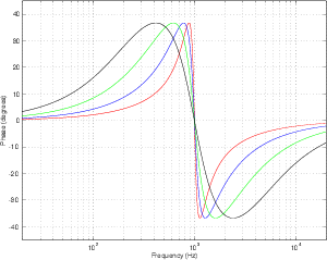
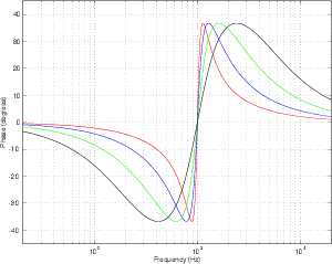
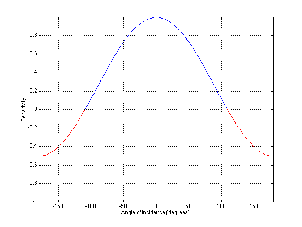
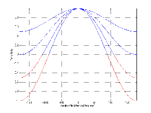
Changes in Q
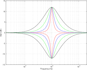
Figures 6.23 and 6.24 shows the difference in gain and phase respectively between
two filters, both with an fc of 1 kHz and a gain of 12 dB and five different Q’s. Again,
one filter calculates Q based on the 3 dB down point, the other based on the midpoint of
the maximum gain.
6.1.7 Further reading
What is a filter? – from Julius O. Smith’s substantial website.
6.2 Compressors, Limiters, Expanders and Gates
6.2.1 What a compressor does.
So you’re out for a drive in your car, listening to some classical music played by an
orchestra on your car’s CD player. The piece starts off very quietly, so you turn up the
volume because you really love this part of the piece and you want to hear it over the
noise of your engine. Then, as the music goes on, it gets louder and louder because that’s
what the composer wanted. The problem is that you’ve got the stereo turned up to
hear the quiet sections, so these new loud sections are really loud – so you turn
down your stereo. Then, the piece gets quiet again, so you turn up the stereo to
compensate.
What you are doing is to manipulate something called the “dynamic range” of the
piece. In this case, the dynamic range is the difference in level between the softest and
the loudest parts of the piece (assuming that you’re not mucking about with the volume
knob). By fiddling with your stereo, you’re making the soft sounds louder and the loud
sounds softer, and therefore compressing the dynamics. The music still appears to have
quiet sections and loud sections, but they’re not as different as they were without your
fiddling.
In essence, this is what a compressor does – at the most basic level, it makes loud
sounds softer and soft sounds louder so that the music going through it has a smaller (or
compressed) dynamic range. Of course, I’m oversimplifying, but we’ll straighten that
out.
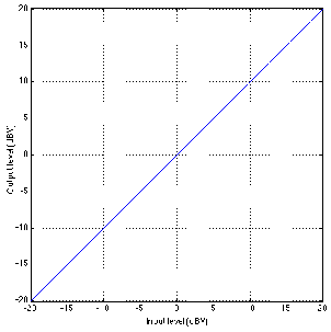
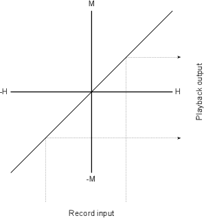
Let’s look at the gain response of an ideal piece of wire. This can be shown as a
transfer function as seen in Figure 6.25.
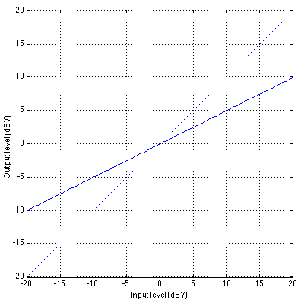
Now, let’s look at the gain response for a simple device that behaves as an
oversimplified compressor. Let’s say that, for a sine wave coming in at 0 dBV (1 Vrms,
remember?) the device has a gain of 1 (or output=input). Let’s also say that, for every 2
dB increase in level at the input, the gain of this device is reduced by 1 dB – so, if
the input level goes up by 2 dB, the output only goes up by 1 dB (because it’s
been reduced by 1 dB, right?) Also, if the level at the input goes down by 2 dB,
the gain of the device comes up by 1 dB, so a 2 dB drop in level at the input
only results in a 1 dB drop in level at the output. This generally makes the soft
sounds louder than when they went in, the loud sounds softer than when they
went in, and anything at 0 dBV come out at exactly the same level as it goes
in.
If we compare the change in level at the input to the change in level at the output, we
have a comparison between the original dynamic range and the new one. This
comparison is expressed as a ratio of the change in input level in decibels to change in
output level in decibels. So, if the output level goes up 1 dB for every 2 dB increase in
level at the input, then we have a 2:1 compression ratio. The higher the compression
ratio, the more the dynamic range is reduced.
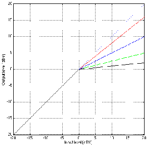
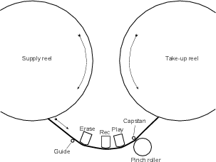
Notice in Figure 6.26 that there is one input level (in this case, 0 dBV) that results in
a gain of 1 – that is to say that the output is equal to the input. That input level is
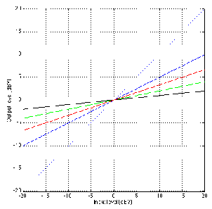
known as the rotation point of the compressor. The reason for this name isn’t
immediately obvious in Figure 6.26, but if we take a look at a number of different
compression ratios plotted on the same graph as in Figure 3, then the reason becomes
clear.
Normally, a compressor doesn’t really behave in the way that’s seen in any of the
above diagrams. If we go back to thinking about listening to the stereo in the car, we
actually leave the volume knob alone most of the time, and only turn it down during the
really loud parts. This is the way we want the compressor to behave. We’d like to
leave the gain at one level (let’s say, at 1) for most of the program material,
but if things get really loud, we’ll start turning down the gain to avoid letting
things get out of hand. The gain response of such a device is shown in Figure
6.28.
The level where we change from being a linear gain device (meaning that the gain of
the device is the same for all input levels) to being a compressor is called the
threshold. Below the threshold, the device applies the same gain to all signal levels.
Above the threhold, the device changes its gain according to the input level. This
sudden bend in the transfer function at the threshold is called the knee in the
response.
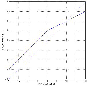
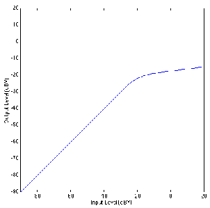
In the case of the plot shown in Figure 6.28, the rotation point of the compressor is
the same as the threshold. This is not necessarily the case, however. If we look at Figure
6.29, we can see an example of a curve where this is illustrated.
This device applies a gain of 5 dB to all signals below the threshold, so an input level
of -20 dBV results in an output of -15 dBV and an input at -10 dBV results in an output
of -5 dBV. Notice that the threshold is still at 0 dBV (because it is the input level over
which the device changes its behaviour). However, now the rotation point is at 10
dBV.
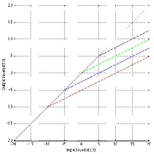
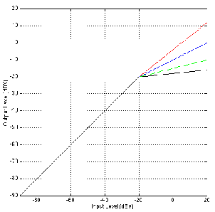
Let’s look at an example of a compressor with a gain of 1 below threshold, a
threshold at 0 dBV and different compression ratios. The various curves for such a device
are shown in Figure 6.30. Notice that, below the threshold, there is no difference in any
of the curves. Above the threshold, however, the various compression ratios result in very
different behaviours.
There are two basic “styles” in compressor design when it comes to the threshold.
Some manufacturers like to give the user control over the threshold level itself, allowing
them to change the level at which the compressor “kicks in.” This type of compressor
typically has a unity gain below threshold, although this isn’t always the case.
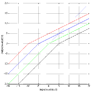
Take a look at Figure 6.31. This shows a number of curves for a device with a
compression ratio of 2:1, unity gain below threshold and an adjustable threshold
level.
The advantage of this design is that the bulk of the signal, which is typically
below the threshold, remains unchanged – by changing the threshold level,
we’re simply changing the level at which we start compressing. This makes the
device fairly intuitive to use, but not necessarily a good design for the final sound
quality.
Let’s think about the response of this device (with a 2:1 compression ratio). If the
threshold is turned up to 12 dBV, then any signal coming in that’s less than 12 dBV will
go out unchanged. If the input signal has a level of 20 dBV, then the output will be 16
dBV, because the input went 8 dB above threshold and the compression ratio is 2:1, so
the output goes up 4 dB.
If the threshold is turned down to -12 dBV, then any signal coming in that’s less than
-12 dBV will go out unchanged. If the input signal has a level of 20 dBV, then the output
will be 4 dBV, because the input went 32 dB above threshold and the compression ratio
is 2:1, so the output goes up 16 dB.
So what? Well, as you can see from Figure 6.31, changing the compression ratio will
affect the output level of the loud stuff by an amount that’s determined by the
relationship between the threshold and the compression ratio.
Consider for a moment how a compressor will be used in a recording situation: we
use the compressor to reduce the dynamic range of the louder parts of the signal. As a
result, we can increase the overall level of the output of the compressor before going to
tape. This is because the spikes in the signal are less scary and we can therefore get
closer to the maximum input level of the recording device. As a result, when we
compress, we typically have a tendency to increase the input level of the device that
follows the compressor. Don’t forget, however, that the compressor itself is adding noise
to the signal, so when we boost the input of the next device in the audio chain, we’re
increasing not only the noise of the signal itself, but the noise of the compressor as well.
How can we reduce or eliminate this problem? Use compressor design philosophy
number 2...
Instead of giving the user control over the threshold, some compressor designers opt
to have a fixed threshold and a variable gain before compression. This has a slightly
different effect on the signal.
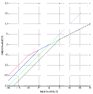
Let’s look at the implications of this configuration using the response in Figure 6.32
which has a fixed threshold of 0 dBV. If we look at the green curve with a gain of 0
dB, then signals coming in are not amplified or attenuated before hitting the
threshold detector. Therefore, signals lower than 0 dBV at the input will be
unaffected by the device (because they aren’t being compressed and the gain is
0 dB). Signals greater than 0 dBV will be compressed at a 2:1 compression
ratio.
Now, let’s look at the blue curve. The low-level signals have a constant 5 dB gain
applied to them – therefore a signal coming in a -20 dBV comes out at -15 dBV. An input
level of -15 dBV results in an output of -10 dBV. If the input level is -5 dBV, a gain of 5
dB is applied and the result of the signal hitting the threshold detector is 0 dBV – the
level of the threshold. Signals above this -5 dBV level (at the input) will be
compressed.
If we just consider things in the theoretical world, applying a 5 dB gain before
compression (with a threshold fixed at 0 dBV) results in the same signal that we’d
get if we didn’t change the gain before compression, reduced the threshold
to -5 dBV and then raised the output gain of the compressor by 5 dB. In the
practical world, however, we are reducing our noise level by applying the gain
before compression, since we aren’t amplifying the noise of the compressor
itself.
There’s at least one manufacturer that takes this idea one step further. Let’s say that
you have the output of a compressor being sent to the input of a recording device. If the
compressor has a variable threshold and you’re looking at the record levels, then the
more you turn down the threshold, the lower the signal going into the recording device
gets. This can be seen by looking at the graph in Figure 6.31 comparing the output levels
of an input signal with a level of 20 dBV. Therefore, the more we turn down the
threshold on the compressor, the more we’re going to turn up the input level on the
recorder.
Take the same situation but use a compressor with a variable gain before
compression. In this case, the more we turn up the gain before compression, the higher
the output is going to get. Now, if we turn up the gain before compression, we are going
to turn down the input level to the recorder to make sure that things don’t get out of
hand.
What would be nice is to have a system where all this gain compensation is done for
you. So, using the example of a compressor with gain before compression: we
turn up the gain before compression by some amount, but at the same time, the
compressor turns down its output to make sure that the compressed part of the
signal doesn’t get any louder. In the case where the compression ratio is 2:1,
if we turn up the gain before compression by 10 dB, then the output has to
be turned down by 5 dB to make this happen. The output attenuation in dB
is equal to the gain before compression (in dB) divided by the compression
ratio.
What would this response look like? It’s shown in Figure 6.33. As you can see,
changes in the gain before compression are compensated so that the output for a signal
above the threshold is always the same, so we don’t have to fiddle with the input level of
the next device in the chain.
If we were to do the same thing using a compressor with a variable threshold, then
we’d have to boost the signal at the output, thus increasing the apparent noise floor of the
compressor and making it sound as bad as it is...
As you can see from Figure 6.33, the advantage of this system is that adjustments in
the gain before compression (or the threshold) don’t have any affect on how the loud
stuff behaves – if you’re past the threshold, you get the same output for the same
input.
Compressor gain characterisitics
So far we’ve been looking at the relationship between the output level and the input level
of a compressor. Let’s look at this relationship in a different way by considering the gain
of the compressor for various signals.
Figure 6.34 shows the level of the output of a compressor with a given threshold and
compression ratio. As we would expect, below the threshold, the output is the same as
the input, therefore the gain for input signals with a level of less than -20 dBV
in this case is 0 dB – unity gain. For signals above this threshold, the higher
the level gets the more the compressor reduces the gain – in fact, in this case,
for every 8 dB increase in the input level, the output increases by only 1 dB,
therefore the compressor reduces its gain by 7 dB for every 8 dB increase. If we
look at this gain vs. the input level, we have a response that is shown in Figure
6.35.
Notice that Figure 6.35 plots the gain in decibels vs. the input level in dBV. The
result of this comparison is that the gain reduction above the threshold appears to be a
linear change with an increase in level. This response could be plotted somewhat
differently as is shown in Figure 6.36.
You’ll now notice that there is a rather dramatic change in gain just above the
threshold for signals that increase in level just a bit. The result of this is an audible gain
change for signals that hover around the threshold – an artifact called pumping This is an
issue that we’ll deal with a little later.
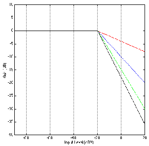
Let’s now consider this same issue for a number of different compression ratios.
Figures 6.37, 6.38 and 6.39 show the relationships of 4 different compression ratios with
the same thresholds and gains before compression to give you an idea of the change in
the gain of the compressor for various ratios.
Soft Knee Compressors
There is a simple solution to the problem of the pumping caused by the sudden change in
gain when the signal level crosses the threshold. Since the problem is caused by the
fact that the gain change is sudden because the knee in the response curve is
a sharp corner, the solution is to soften the sharp corner into a gradual bend.
This response is called a soft knee for obvious reasons as can be seen in Figure
6.40.
Signal level detection
So far, we’ve been looking at a device that alters its gain according to the input level, but
we’ve been talking in terms of the input level being measured in dBV – therefore, we’re
thinking of the signal level in VRMS. In fact, there are two types of level detection
available – compressors can either respond to the RMS value of the input signal, or the
peak value of the input signal. In fact, some compressors give you the option
of selecting some combination of the two instead of just selecting one or the
other.
Probably the simplest signal detection method is the RMS option. As we’ll see later,
the signal that is input to the device goes to two circuits: one is the circuit that changes
the gain of the signal and sends it out the output of the device. The second,
known as the control path determines the RMS level of the signal and outputs a
control signal that changes the gain of the first circuit. In this case, the speed at
which the control circuit can respond to changes in level depends on the time
constant of the RMS detector built into it. For more info on time constants of
RMS measurements, see Section 2.1.6. The thing to remember is that an RMS
measurement is an average of the signal over a given period of time, therefore the
detection system needs a little time to respond to the change in the signal. Also,
remember that if the time constant of the RMS detection is long, then a short,
high level transient will get through the system without it even knowing that it
happened.
If you’d like your compressor to respond a little more quickly to the changes in signal
level, you can typically choose to have it determine its gain based on the peak level of the
signal rather than the RMS value. In reality, the compressor is not continuously looking
at the instantaneous level of the voltage at the input – it’s usually got a circuit built in that
looks at a smoothed version of the absolute value of the signal. Almost all compressors
these days give you the option to switch between a peak and an RMS detection
circuit.
On high-end units, you can have your detection circuit respond to some mix of the
simultaneous peak and RMS values of the input level. Remember from Chapter 2.1.6
that the ratio of the peak to the RMS is called the crest factor. This ratio of
peak/RMS can either be written as a value from 0 to something big, or it may be
converted into a dB scale. Remember that, if the crest factor is near 0 (or -∞
dB), then the RMS value is much greater than the peak value and therefore the
compressor is responding to the RMS of the signal level. If the crest factor is a
big number, then the compressor is responding to the peak value of the input
level.
Time Response: Attack and Release
Now that we’re talking about the RMS and the smoothed peak of the signal, we
have to start considering what time it is. Up to now, we’ve been only looking
at the output level or the gain of the compressor based on a static input level.
We have been assuming that the only thing we’re sending through the unit is a
steady-state sine tone. Of course, this is pretty boring to listen to, but if we’re going to
look at real-world signals, then the behaviour of the compressor gets pretty
complicated.
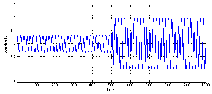
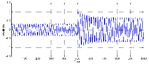
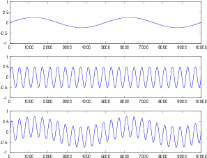
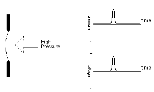
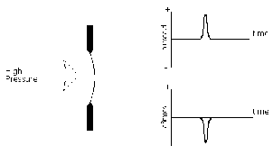
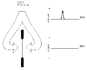
Let’s start by considering a signal that’s quiet to begin with and suddenly gets louder.
For the purposes of this discussion, we’ll simulate this with a pulse-modulated sine wave
like the one shown in Figure 6.41.
Unfortunately, a real-world compressor cannot respond instantaneously to this
sudden change in level. In order to be able to do this, the unit would have to be able to
see into the future to know what the new peak value of the signal will be before we
actually hit that peak. (In fact, some digital compressors can do this by delaying the
signal and turning the present into the past and the future into the present, but we’ll
pretend that this isn’t happening for now...).
Let’s say that we have a compressor with a gain before compression of 0 dB and a
threshold that’s set to a level that’s higher than the lower-level signal in Figure 6.41, but
lower than the higher-level signal. So, the first part of the signal, the quiet part, won’t be
compressed and the later, louder part will. Therefore the compressor will have to have a
gain of 1 (or 0 dB) for the quiet signal and then a reduced gain for the louder
signal.
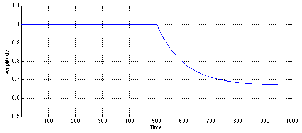
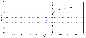
Since the compressor can’t see into the future, it will respond somewhat slowly to the
sudden change in level. In fact, most compressors allow you to control the speed with
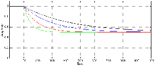
which the gain change happens. This is called the attack time of the compressor. Looking
at Figure 6.42, we can see that the compressor has a sudden awareness of the new
level (at Time = 500) but it then settles gradually to the new gain for the higher
signal level. This raises a question – the gain starts changing at a known time,
but, as you can see in Figure 6.42, it approaches the final gain forever without
really reaching it. The question that’s raised is “what is the time of the attack
time?” In other words, if I say that the compressor has an attack time of 200
ms, then what is the relationship between that amount of time and the gain
applied by the compressor. The answer to this question is found in the chapter on
capacitors. Remember that, in a simple RC circuit, the capacitor charges to a new
voltage level at a rate determined by the time constant which is the product
of the resistance and the capacitance. After 1 time constant, the capacitor has
charged to 63 % of the voltage being applied to the circuit. After 5 time constants,
the capacitor has charged to over 99 % of the voltage, and we consider it to
have reached its destination. The same numbers apply to compressors. In the
case of an attack time of 200 ms, then after 200 ms has passed, the gain of the
compressor will be at 63 % of the final gain level. After 5 times the attack time
(in this case, 1 second) we can consider the device to have reached its final
gain level. (In fact, it never reaches it, it just gets closer and closer and closer
forever...)
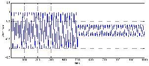
What is the result of the attack time on the output of the compressor? This actually is
pretty interesting. Take a look at Figure 6.43 showing the output of a compressor that has
the signal in Figure 6.41 sent into it and responding with the gain in Figure 6.42. Notice
that the lower-level signal goes out exactly as it went it. We would expect this because
the gain of the compressor for that portion of the signal is 1. Then the signal suddenly
increases to a new level. Since the compressor detection circuit take a little while
to figure out that the signal has gotten louder, the initial new loud signal gets
through, almost unchanged. As we get further and further into the new level in
time, however, the gain settles to the new value and the signal is compressed
as we would expect. The interesting thing to note here is that a portion of the
high-level signal gets through the compressor. The result is that we’ve created a
signal that sounds like more of a transient than the input. This is somewhat
contrary to the way most people tend to think that a compressor behaves. The
common belief is that a compressor will control all of your high-level signals, thus
reducing your dynamic range – but this is not exactly the case as we can see in
this example. In fact, it may be possible that the perceived dynamic range is
greater than the original because of the accents on the transient material in the
signal.
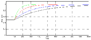
Similarly, what happens when the signals decreases in level from one that is being
compressed to one that is lower than the threshold? Again, it takes some time for the
compressor’s detection circuit to realize that the level has changed and therefore
responds slowly to fast changes. This response time is called the release time of the
compressor. (Note that the release time is measured in the same way as the attack time –
it’s the amount of time it takes the compressor to get to 63% of its intended
gain.)
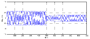
For example, we’ll assume that the signal in Figure 6.44 is being fed into a
compressor. We’ll also assume that the higher-level signal is above the compression
threshold and the lower-level signal is lower than the threshold.
This signal will result in a gain reduction for the first part of the signal and no gain
reduction for the latter part, however, the release time of the compressor results in a
transition time from these two states as is shown in Figure 6.45.
Again, the result of this gain response curve is somewhat interesting. The output of
the compressor will start with a gain-reduced version of the louder signal. When the
signal drops to the lower level, however, the compressor is still reducing the gain for a
while, therefore we wind up with a compressed signal that’s below the threshold – a
signal that normally wouldn’t be compressed. As the compressor figures out that the
signal has dropped, it releases its gain to return to a unity gain, resulting in an output
signal shown in Figure 6.46.
Just for comparison purposes, Figures 6.47 and 6.48 show a number of different
attack and release times.
One last thing to discuss is a small issue in low-cost RMS-based compressors. In
these machines, the attack and release times of the compressor are determined by the
time constant of the RMS detection circuit. Therefore, the attack and release times are
identical (normally, we call them “symmetrical”) and not adjustable. Check your manual
to see if, by going into RMS mode, you’re defeating the attack time and release time
controls.
6.2.2 The Nitty-Gritty
Level detection - The awful truth
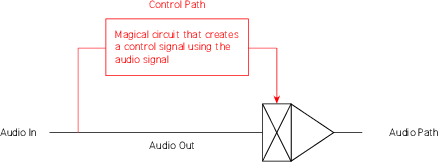
On its simplest level, a compressor can be thought of as a device which controls its gain
based on the incoming signal. In order to do this, it takes the incoming audio and sends it
in two directions, along the audio path, which is where the signal goes in, gets modified
and comes out the output; and the control path, (also known as a side chain) where the
signal comes in, gets analysed and converted into a different signal which is used to
control the gain of the audio path.
As a result, we can think of a basic compressor as is shown in the block diagram in
Figure 6.49.
If we’re going to start asking difficult questions about compressors, a good place to
start is to look at the the behaviour of the level detection component of the side
chain. Exactly what kind of level is the level detection measuring (or at least,
claiming to measure...), how accurate is that measurement, and how well does it
behave?
There are a number of possible answers to the first part of the question. Depending
on the compressor, you might have one with an RMS detector, a peak detector (probably
with an RC-based attack and release control) or a pseudo-RMS detector. Let’s look at
how each of these behaves, how they behave differently, and how neither of them will
give you what you expect or want...
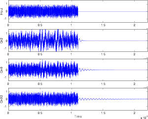
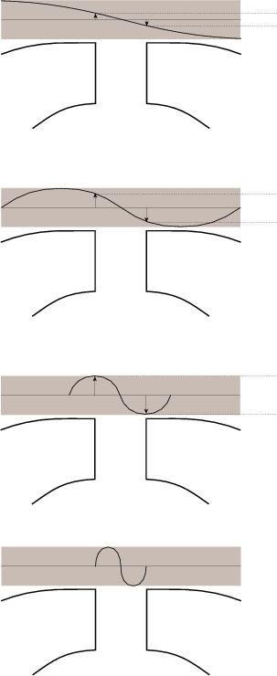
Let’s start by looking at a very simple signal. We will make a stepped signal that goes
from 0 V
to 0.5 V to 1 V, back down to 0.5 V and returning to (almost) 0 V. This input signal is
shown as the green line in Figures 6.50 to 6.57.
RMS Detectors
Figures 6.50 and 6.51 show the response of a running RMS measurement
of the signal. There are at least four things to notice here. Firstly, when the
input voltage changes, the RMS measurement is always a little late getting to
the new value. (To be precise, the amount of time it takes to get to the new
voltage is equal to the RMS time window.) Secondly, the shapes of the attack and
the decay of the RMS detector output are symmetrical. Thirdly, there are two
discontinuities in the slope of the RMS detector output signal on each change of
input voltage. (In other words, there are two “corners” in the black line for
every jump in the green line.) Fourthly, because this is a DC signal (between
changes, at least...) the RMS output is equal to the input after the detector has
settled. This would not be true if the input voltage was changing faster than one
RMS time constant apart. If that were the case, then the RMS detector would
not have time to get to the new input voltage before it had to go somewhere
else. Later, we’ll see that this is a problem with more musical signals like sine
waves.
Pseudo RMS Detectors
Some manufacturers don’t like implementing true RMS detection in their
compressors because it’s expensive. If you’re working with analogue gear, it means you
have to put in more parts. If you’re building a digital compressor, then you need more
memory. Either way, if you can get a nearly-RMS behaviour without the added expense,
you might try to get away with this. One easy way to do this is to keep the R and the S
and throw away the M in the RMS. In other words, you Square the input signal, then
low-pass filter the result with a first-order RC filter (instead of finding the Mean value),
and get the square Root of the result. If you’re reasonably careful about your RC time
constant (in other words, the cutoff frequency of your low-pass filter), then you
can get something that behaves something like an RMS detector without the
expense.
However, what you get will not be exactly like an RMS detector as we can see in
Figures 6.52 and 6.53.
Note that there is a small difference in the ramp-up behaviour as compared to a
true-RMS detector. Specifically, there is only one discontinuity in the signal’s slope (only
one corner in the black line). Other than that, it appears to be almost the same shape.
However, the ramp-down behaviour is very different. If you look at the shape of the
curve in Figure 6.52 compared to Figure 6.50, you can see that they have sort of an
opposite behaviour in time. Where the RMS detector has a an increasingly vertical slope
as it goes through its decay, the pseudo-RMS detector starts with a nearly-vertical slope
and becomes more and more horizontal at it reaches its target value. This difference is
even more evident when you take a look at the same curves displayed on a
decibel scale. (see Figures 6.51 and 6.53.) The RMS detector’s output has an
increasingly vertical decay when measured in decibels (therefore the rate of change
in dB increases over time) whereas the pseudo-RMS detector’s output has a
constant slope in dB over time. (This means that the decay of the pseudo-RMS
detector’s output is more like the decay of a musical instrument or a reverb
tail.)
Peak Detector with Symmetrical RC-based Attack and Release
In other cases, a compressor will be based on a peak detection circuit which is
typically followed by a first-order RC circuit to control the attack and release times. In
this case, the absolute value of the incoming signal is low-pass filtered by the first-order
low-pass filter. Usually there are two different filters - one for attack and the other for the
release. However, we’ll look at a system with a single low-pass first. Figures 6.54 and
6.55 show the output of a peak detector with a single RC filter used to smooth its
output.
Note that the behaviour of this circuit is very similar to that of the pseudo-RMS
detection circuit. In fact, if you don’t look carefully, you’ll think that the two curves are
identical. However, they’re not – looking carefully, you’ll see that the response of the
peak detector with the symmetrical RC low-pass is faster than that of the pseudo-RMS
detector. This is particularly noticeable in the decibel scale representations of the
responses in Figures 6.55 and 6.53. This is due to the fact that, in the case of the
pseudo-RMS detector, the RC circuit is applied to the square of the signal (analogous to
the signal’s power) whereas, in the case of the peak detector, the RC circuit is
applied to the absolute value of the signal. This means, that, in the case of the
pseudo-RMS detector, we’re seeing the square root of the response of the RC filter,
whereas in the case of the peak detector, we see the unaltered response of the RC
filter.
Peak Detector with Asymmetrical Attack and Release
Of course, it is more normal with a peak compressor to have separate attack and
release time controls. While this will typically be implemented in almost exactly the
same way as the previously-described circuit with a symmetrical attack and
release, the usual setting of fast-attack-with-a-slow-release may result in an
effect of this circuit to be seen more often. Figures 6.56 and 6.57 show a peak
detector with separate RC smoothing filters for the attack and the release. The
attack filter (when the input signal is increasing) is set to have a time constant
of 0.2 ms, identical to the symmetrical filter shown above. The release filter
(when the input signal is decreasing) is set to have a time constant of 100 times
the attack. Note that these values should not be taken as suggestions – they
are merely arbitrary values chosen to illustrate the behaviour of the detection
circuit.
As can be seen in Figures 6.56 and 6.57, the attack of the detection circuit is identical
to the symmetrical behaviour shown in Figures 6.54 and 6.55. This is because
the two circuits are, in fact identical. However, as is immediately obvious in
both Figure 6.56 and Figure 6.57, the release takes much longer to decay. This
should not come as a surprise. However, the interesting thing to note is the
change in slope at 35 ms. This is caused by the fact that the target value (the
input voltage) changes at 35 ms, before the decay from the change at 25 ms has
settled.
Sine waves
Let’s now move away from a simple input signal (the stepped DC used above) to
something a little more complicated like a sine wave. This makes the detectors a little
more busy, since they’re always trying to catch up to an ever-changing input level. Now
the behaviour of the detectors’ outputs will be highly dependent on the relationship
between the input signal’s period and the time constant of the detectors’ smoothing
filters.
When the period of the input signal is much longer than the detector’s time constant,
the level detector will have an output that is very similar to the absolute value of the
input signal. This can be seen in the example in Figure 6.58. As can be seen in
this example, nearly all of the detectors’ outputs are equivalent, the exception
being the Peak Detector with the asymmetrical attack and release, since its
release time constant is 20 ms – two times the period of the incoming signal.
In the other three cases, it can be seen that the output of the detectors swings
back and forth from nearly 0 V up to a value very close to the peak value of
the input signal. We can think of this deviation as a ripple in the outputs of
the detectors. So, we can say that, when the period of the input signal is much
greater than the time constant of the detector’s smoothing filter, the peak-to-peak
ripple on the output of the detector is close to the peak amplitude of the input
signal.
In addition, you can see that the outputs of all level detectors is slightly behind the
input signal – some more than others.
As the period of the input signal decreases and approaches the time constant of the
level detector, the ripple on the output of the detector will decrease. An example of this is
shown in Figure 6.59. In almost all cases shown in this plot, the ripple follows the
envelope of the absolute value of the signal, however, in all cases, that ripple has a
much smaller peak-to-peak amplitude than we saw in the case of the 100 Hz
input.
You may notice that there is an exception. After it has stabilised following the initial
start of the sine wave, the RMS detector has no ripple. This is because the period of the
input signal is equal to the RMS time window in this example. (In fact, as we’ll see
later, this will happen at other specific frequencies – whenever the RMS time
window is exactly equal to 0.5 periods, 1 period, 1.5 periods, 2 periods, and so
on...)
When the period of the input signal is much shorter than the time constant of the
smoothing filter of the detector, the ripple of the detectors becomes even smaller,
and their attack behaviour at the onset of the input sine wave is more similar
to the attack behaviour with a stepped DC signal. This can be seen in Figure
6.60
Figures 6.61, 6.62 and 6.63 are included to show the release behaviour of the various
detectors at the end of the same sine wave inputs. Note in Figure 6.61 that, like the signal
itself, the RMS detector has a corner in its output when it reaches 0, whereas the other
detectors have a smooth transition to 0.
In Figure 6.62 we can see that the release envelope of the RMS detector is exactly
symmetrical to the attack envelope (shown in Figure 6.59). In fact, this is true for other
frequencies – it’s just easier to see here...
Again in Figure 6.63 we can see that, at very high frequencies when the signal’s
period is much shorter than the detector’s smoothing filter’s time constant, the release
behaviour of the various detectors is very similar to that seen in the case of an input
signal made with a stepped DC.
Now that we’ve seen some examples of the ripple of the output of the various level
detectors at three frequencies, we can look at the magnitude of the ripple across a wider
frequency range. Figure 6.64 shows the minimum and maximum output levels from the
four detectors we’ve been looking at previously. The input signal is a sine wave with a
peak amplitude of 1. The RMS time window is 1 ms. The RC time constant of the low
pass filters used in the pseudo-RMS detector, the peak detector with the symmetrical
attack and release, and the attack of the asymmetrical peak detector is 0.2 ms.
The RC time constant of the release of the asymmetrical peak detector is 20
ms.
At very low frequencies, you can see that the differences between the minimum and
maximum outputs from the detectors is largest. This is because, as we saw in Figure
6.58, the outputs of all of the detectors (excepting the peak detector with the long release
time) is nearly the same as the absolute value of the input signal. As the signal goes
up and down, so does the output of the detector. This appears in the graphs in
Figures 6.64 and 6.65 as large differences in the maximum and minimum output
levels.
As the frequency of the input signal goes up, the difference between the maximum
and minimum levels of the outputs of the detectors decreases. In the case of the peak
detector with the long release time, the two values converge on a level very
near the peak level of the input signal. The pseudo-RMS and the symmetrical
peak detector both converge on levels around 3 dB below the peak level of
the signal. The odd one is the RMS detector. As you can see, at 500 Hz, the
minimum and maximum levels of the output of the RMS detector are the same -
at -3.01 dB relative to the peak level of the input. This means that there is no
ripple in the output of the RMS detector at this particular frequency (where the
period of the input signal is exactly two times the RMS time window). As we
go slightly above 500 Hz, the maximum output of the RMS detector’s output
increases and the minimum level decreases – in other words, the ripple in its output
re-appears. At 1 kHz (when the period of the input signal is the same as the RMS
time window) there is no ripple again... This behaviour repeats as we go up in
frequency.
Why does the output of the RMS detector have no ripple at some frequencies and
ripple at others? Let’s look at two signals as they sit in the RMS detector’s time
window. Figure6.66 shows a signal with a period of exactly one RMS time
window. The signal is the black sine wave. Four RMS time windows are shown,
each at a different time (the 4 blue boxes). For each RMS time window, its
RMS value is shown as a horizontal red line. There are two things to notice
here. Firstly, the sine wave fits exactly in the boxes, therefore, each box has
identical contents. This would be true regardless of where in the sine wave you are.
Secondly, notice that the red lines all have the same value – this is because the
output of the RMS window is stable, so there is no ripple in its output at this
frequency.
Now compare this to the plot in Figure 6.67 which is the same as Figure 6.66, but
with a slightly higher frequency. The length of the RMS time window is the same in both
plots. Now you can see that the contents of the four different RMS time windows at
different times in the sine wave are not the same, therefore their outputs are
also different. This accounts for the ripple in the RMS detector output at this
frequency.
Figures 6.64 and 6.65 show the results of a specific group of detectors with specific
frequencies. This is useful for getting an intuitive understanding of the behaviours of
the different detectors, but it’s not very useful if you have a detector with a
different time constant or time window. Figures 6.68 and 6.69 show the same
information in a more generalised form. In these, instead of the frequency on
the x-axis, the ratio of the signal’s period to the RMS time window and the
RC time constants. If these are confusing, just look at Figures 6.64 and 6.65
instead.
To now, we’ve been looking at the maximum and minimum output levels from the
different detectors, however, these can be simplified into a single value stating the
peak-to-peak ripple of the output of each detector. This is simply the vertical distance
between the two plots for each detector in, for example, Figure 6.69. This version
of displaying the same information is shown in Figures 6.70, 6.71, 6.72, and
6.73.
Another way to look at the behaviour of these level detectors is to consider the error
of the measurement that they provide. This is simply the difference between the value
given by the output of the detector and the value that we know is actually the right
answer. In this case, we know that we sent in a sine wave with a peak amplitude of 1 (and
therefore an RMS of 1∕ ) at all frequencies. So, these are the values we expect to see
coming out of the level detectors (1 for the peak detectors, 1∕
) at all frequencies. So, these are the values we expect to see
coming out of the level detectors (1 for the peak detectors, 1∕ for the RMS
detectors).
for the RMS
detectors).
As we already know, the outputs of all of the detectors are not constant over time, so
we cannot really evaluate the real error. All we can do is look, as it bobs up and
down, how close it is to the correct answer. These is shown in Figures 6.74 to
6.81.
Be wary of these plots, however... Although it looks like the peak detector
with the separate attack and release times is the most accurate of the detectors
shown here, this is only true after it has settled. As you can see, way back in
Figure 6.60 this detector has the longest response time of the four detectors
analysed here, so it takes more time to be right. Then again, you could argue
that the other detectors are earlier, just more inaccurate... Would you rather
have the right answer too late, or the wrong answer now? The choice is up to
you...
6.2.3 How compressors compress
Take a look back to the simplified block diagram of a compressor shown in Figure 6.49.
Notice that the input gets split in two directions right away, going to the two different
paths.
At the heart of the audio path is a device we have’t seen before – it’s drawn in block
diagrams (and sometimes in schematics) as a triangle (so we know right away it’s an
amplifier of some kind) attached to a box with an “X” through it on the left.
This device is called a voltage controlled amplifier or VCA. It has one audio
input on the left, one audio output on the right and a control voltage (or CV)
input on the top. The amplifier has a gain which is determined by the level of
the control voltage. This gain is typically applied to the current through the
VCA, not the voltage – this is a new concept as well... but we’ll get to that
later.
If you go to the VCA store and buy a VCA, you’ll find out that it has an interesting
characteristic. Usually, it will have a logarithmic change in gain for a linear change in
voltage at the control voltage input. For example, one particular VCA from
THAT corporation has a gain of 0 dB (so input = output) if the CV is at 0 V.
If you increase the CV by 6 mV, then the gain of the VCA goes down by 1
dB.
So, for that particular VCA, we could make Table 6.3 which we’ll use later.
|
|
| Control Voltage (mV) | Gain of Audio signal (dB) |
|
|
| -12 | +2 |
| -6 | +1 |
| 0 | 0 |
| +6 | -1 |
| +12 | -2 |
|
|
| |
Table 6.3: The relationship between the control voltage and the gain applied to
the audio signal for the hypothetical VCA shown in Figure 6.49
The only problem with the schematic so far is that the VCA is a current
amplifier not a voltage amplifer. Since we prefer to think in terms of voltage
most of the time, we’ll need to convert the voltage signal that we’re feeding
into the compressor into a current signal of the same shape. This is done by
sticking the VCA in the middle of an inverting amplifier circuit as shown in Figure
6.82:
Here’s an explanation of why we have to build the circuit like this. Remember back
to the first stuff on op amps – one of the results of the feedback loop is that the voltage
level at the negative input leg MUST be the same as the positive input leg. If this wasn’t
the case, then the huge gain of the op amp would result in a clipped output. So, we
call the voltage level at the negative input “virtual ground” because it has the
same voltage level as ground, but there’s really no direct connection to ground.
If we assume that the VCA has an impedance through it of 0Ω (a pretty safe
assumption), then the voltage level at the signal input of the VCA is also the same
as ground. Therefore the current through the resistor on the left in the above
schematic is equal to the “Audio in” voltage divided by the resistor value. Now, if
we assume that the VCA has a gain of 0 dB, then the current coming out of it
equals the current going into it. We also happen to remember that the input
impedance of the op amp is infinite, therefore all the current on the wire coming out
of the VCA must go through the resistor in the feedback loop of the op amp.
This results in a voltage drop across it equal to the current multiplied by the
resistance.
Let’s use an example. If the “Audio in” is 1 Vrms, then the current through the input
resistor on the left is 0.1 mArms. That current goes through the VCA (which we’ll
assume for now has a gain of 0 dB) and continues on through the feedback
resistor. Since the current is 0.1 mA rms and the resistor is 10 kΩ, then the
voltage drop across it is 1 V rms. Therefore, the “Audio out” is 1 V rms but
opposite in polarity to the input. This is exactly the same as if the VCA was not
there.
Now take a case where the VCA has a gain of +6 dB for some reason. The voltage
level at its input is 0 V (virtual ground) so the current through the input resistor is still 0.1
mA rms (for a 1 V rms input signal). That current gets multiplied by 2 in the VCA
(because it has a gain of +6 dB) making it 0.2 mA rms. This all goes through the
feedback resistor which results in a voltage drop of 10k * 0.2 mArms = 2 V rms (and
opposite in polarity). Ah hah! The gain applied to the current by the VCA now shows up
as a gain on the voltage at the output. Now all we need to do is to build the control
circuitry and we have a compressor...
The control circuitry needs a number of things: a level detector, compression
ratio adjustment, threshold, threshold level adjustment and some other stuff that
we’ll get to. We’ll take them one at a time. For now, let’s assume that we have a
compressor which is only looking at the RMS level to determine its compression
characteristics.
RMS Detector
This is an easy one. You buy a chip called an RMS detector. There’s more stuff to do
once you buy that chip to make it happy, but you can just follow the manufacturer’s
specifications on that one. This chip will give you a DC voltage output which is
determined by the logarithmic level of an AC input. For example, using a THAT Corp.
chip again... The audio input of the chip is measured relative to 0.316 V rms (which
happens to be -10 dBV). If the RMS level of the audio input of the chip is 0.316 V rms,
then the output of the chip is 0 V DC. If you increase the level of the input
signal by 1 dB, the output level goes up by 6 mV. Conversely, if the input level
goes down by 1 dB, then the output goes down by 6 mV. An important thing to
notice here is that a logarithmic change in the input level results in a linear
change in the output voltage. So, we build another table for future reference
again:
|
|
| Input level (dBV) | Output Voltage (mV) |
|
|
| -8 | +12 |
| -9 | +6 |
| -10 | 0 |
| -11 | -6 |
| -12 | -12 |
|
|
| |
Table 6.4: The relationship between the input level and the output voltage for the
hypothetical RMS detector in Figure 6.83
Now, what would happen if we took the output from this RMS detector and
connected it directly to the control voltage input of the VCA like in the diagram in Figure
6.83?
Well, if the input level to the whole circuit was -10 dBV, then the RMS detector
would output a 0 V control voltage to the CV input of the VCA. This would cause it to
have a gain of 0 dB and its output would be -10 dBV. BUT, if the input was -11 dBV,
then the RMS detector output would be -6 mV making the VCA gain go up
by 1 dB, raising the output level to -10 dBV. If the input level was -9 dBV,
then the RMS detector’s output goes to 6 mV and the VCA gain goes to -1
dB, so the output is -10 dBV. Essentially, no matter what the input level was,
the output level would always be the same. That’s a compression ratio of ∞ :
1.
Although the circuit above would indeed compress with a ratio of ∞ : 1, that’s not
terribly useful to us for a number of reasons. Let’s talk about how to reduce the
compression ratio. Take a look at the circuit in Figure 6.84.
If the potentiometer has a linear scale, and the wiper is half-way up the pot,
then the voltage at the wiper is one half the voltage applied to the top of the
pot. This means, in turn, that the voltage applied to the CV input of the VCA
is one half the voltage output from the RMS detector. How does this effect
us? Well, if the input level of the circuit is -10 dBV, then the RMS detector
outputs 0 V, the wiper on the pot is at 0 V and the gain of the VCA is 0 dB,
therefore the output level is -10 dBV. If, however, the input level goes up by 1
dB (to -9 dBV), then the RMS detector output goes up by 6 mV, the wiper on
the pot goes up by 3 mV, therefore the gain of the VCA goes down by 0.5 dB
and the output level is -9.5 dB. So, for a 2 dB change in level at the input, we
get a 1 dB change in level at the output – in other words, a 2:1 compression
ratio.
If we put the pot at another location, we change the ratio of the voltage at the top of
the pot (which is dependent on the input level to the RMS detector) to the gain (which is
controlled by the wiper voltage). So, we have a variable compression ratio from 1:1 (no
compression) to infinity:1 (complete limiting) and a rotation point at -10 dBV. This is
moderately useful, but real compressors have a threshold. So – how do we make this
happen?
Threshold
The first thing we’ll need to make a threshold detection circuit is a way of looking at the
signal and dividing it into a low voltage area (in which nothing gets out of the circuit)
and a high area (in which the output = the input to the circuit). We already looked at
how to do this in a rather crude fashion – it’s called a half-wave rectifier. Since
the voltage of the wiper on the pot is going positive and negative as the input
signal goes up and down respectively, all we need to do is rectify the signal after
the wiper so that none of the negative voltage gets through to the CV input
of the VCA. That way, when the signal is low, the gain of the VCA will be 0
dB, leaving the signal unaffected. When the signal goes positive, the rectifier
lets the signal through, the gain of the VCA goes down and the compressor
compresses.
One way to do this would simply be to put a diode in the circuit pointing away from
the wiper. This wouldn’t work very well because the diode would need the 0.7 V
difference across it to turn on in the first place. Also, the turn-on voltage of the
diode is a little sloppy, so we wouldn’t know exactly what the threshold was
(but we’ll come back to this later). what we need then, is something called a
precision rectifier – a circuit that looks like a perfect diode. This is pretty easy to
build with a couple of diodes and an op amp as is shown in the circuit in Figure
6.85.
Notice that the circuit has two effects – the first is that it is a half-wave rectifier, so
only the positive half of the input gets through. The second is that it is an inverting
amplifier, so the output is opposite in polarity to the input – therefore, in order to get
things back in the right polarity, we’ll have to flip the polarity once again with a second
inverting amplifier with unity gain.
If we add this circuit between the wiper and the VCA CV input like the diagram
shown in Figure 6.86, what will happen?
Now, if the input level is -10 dBV or lower, the output of the RMS detector is 0 V or
lower. This will result in the output of the half-wave rectifier being 0 V. This will
be multiplied by -1 in the polarity inversion, resulting in a level of 0 V at the
CV input of the VCA. This means that if the input signal is -10 dBV or lower,
there is no gain change. If, however, the input level goes above -10 dBV, then
the output of the RMS detector goes up. This gets through the rectifier and
comes out multiplied by -1, so for every increase in 1 dB above -10 dBV at the
input, the output of the rectifier goes DOWN by an amount determined by the
position of the wiper. This is multiplied by -1 again at the polarity inversion
and sent to the CV input of the VCA causing a gain change. So, we have a
threshold at -10 dBV at the input. But, what if we wanted to change the threshold
level?
In order to change the threshold level, we have to trick the threshold detection circuit
into thinking that the signal has reached the threshold before it really has. Remember that
the output of the RMS detection circuit (and therefore the wiper on the pot) is DC (well,
technically speaking, it varies if the input signal’s RMS level varies, but we’ll say it’s DC
for now). So, we need to mix some DC with this level to give the input to the
rectification circuit an additional boost. For example, up until now, the threshold is -10
dBV at the input because that’s where the output of the RMS detector crosses
from negative to positive voltage. If we wanted to make the threshold -20 dBV,
then we’d need to find out the output of the RMS detector if the signal was -20
dBV (that would be -60 mV because it’s 6 mV per dB and 10 dB below -10
dBV) and add that much DC voltage to the signal before sending it into the
rectification stage. There are a couple of ways to do this, but one efficient way is to
combine an inverting mixer circuit with the half-wave rectifier that’s already
there.
The threshold level adjustment is just a controllable DC level which is mixed with
the DC level coming out of the RMS detector. One important thing to note is that
when you turn UP this level to the top of the pot, you are actually getting a
lower voltage (notice that the top of the pot is connected to a negative voltage
supply). Why is this? Well, if the output of the threshold level adjustment wiper
is 0 V, this gets added to the RMS detector output and the threshold stays at
-10 dBV. If the output of the threshold level adjustment wiper goes positive,
then the output of the RMS detector is increased and the rectifier opens up at a
lower level, so by turning UP the voltage level of the threshold adjustment pot,
you turn DOWN the threshold. Of course, the size of the change we’re talking
about on the threshold level adjustment is on the order of mV to match the level
coming out of the RMS detector, so you might want to be sure to make the
maximum and minimum values possible from the pot pretty small. See the THAT
Corp .pdf file linked at the bottom of the page for more details on how to do
this.
So, now we have a compressor with a controllable compression ratio and a threshold
with a controllable level. All we need to do is to add an output gain knob. This is pretty
easy since all we’re going to do is add a static gain value for the VCA. This can be done
in a number of ways, but we’ll just add another DC voltage to the control voltage after
the threshold. That way, no matter what comes out of the threshold, we can alter the
level.
The diagram in Figure 6.88 shows the whole circuit. Note that the output gain control
has the + DC voltage at the top of the pot. This is because it will become negative after
going through the polarity inversion stage, making the VCA go up in gain. Since this DC
voltage level is added to the control voltage signal after the threshold detection circuit,
it’s always on – therefore it’s basically the same as an output level knob. In fact, it is an
output level knob.
Everything I’ve said here is basically a lead-up to the pdf file below from THAT
Corp. It’s a good introduction to how a simple RMS-based compressor works. It includes
all the response graphs that I left out here, and goes a little further to explain how to
include a soft knee for your circuit. Definitely recommended reading if you’re planning
on learning more about these things...
6.2.4 Suggested Reading List
Basic Compressor/Limiter Design – from THAT Corporation www.thatcorp.com/datashts/an100a.pdf
Users Manual for the GML 8900 Dynamic Range Controller www.gmlinc.com/8900.pdf
6.3 Analog Tape
6.3.1 The simple story
Once upon a time when you were a kid, you probably did a science experiment where
you made a compass using a tray of water and a sewing needle. The only work involved
in the experiment was to turn the needle into a magnet by stroking it over and over with a
permanent magnet. The lesson here is that if you put a piece of iron in a magnetic field,
you can turn it into a magnet.
Let’s make soup! Unfortunately, not a good French onion soup, or a seafood
chowder, however... We’ll make a slurry of little needles (usually called a magnetic oxide
because it’s made out of things like ferric oxide, for example) suspended in a
non-magnetic liquid binder. We’ll then pour this goo on a wide sheet of polyester and let
it dry so that the little needles are stuck to the sheet. Just before we dry it, we
run the polyester with the goo on it through a really strong magnetic field so
all the needles are pointing in the same direction – just like little compasses.
Eventually, we’re going to roll up this sheet, so we’ll put a carbon coating on the
back of it so that it’s slippery and it doesn’t build up static electricity. Then
we take the wide sheet and slice it into strips ranging from 0.125 to 2 inches
wide.
A cross section of this stuff looks like Figure 6.89
The important thing about the magnetic oxide coating on the polyester is that it is
pretty easy to magnetize. If we put it in a strong magnetic field and then take it out, it will
maintain that field in the coating, just like the needle that we magnetized to make a
compass back when we were kids.
So, how do we magnetize the coating? We already know two useful things
from Section 2.6: the first is that if we run current through a wire, we get a
magnetic field around it. The second is that, if that wire is coiled around an iron
bar, the iron bar will act like a magnet. So, let’s take an iron bar and bend it so
that the two ends almost touch each other. We’ll also coil a wire around it so
that the whole thing looks like Figure 6.90. This is a very basic model of a
record head of an analog tape recorder. (Actually, it also works as a playback
head.)
When we put current in the coil, the iron bar it’s coiled around temporarily becomes
a magnet. This, in turn, causes magnetic lines of force to go from one end of the bar to
the other across the narrow gap that we created (seen at the top in Figure 6.90. If we look
at a close-up of those magnetic lines of force, we’d see something like Figure
6.91.
In its most simple form, if we send an audio signal into the coil of wire wrapped
around the tape head, we’ll cause the magnetic field to change in strength and polarity at
the gap of the record head. If we leave the magnetic tape sitting on the head while this
happens, we’ll be causing that magnetic field to be stored on the tape. If we want to keep
the magnetic field stored on the tape, then we’ll move it away from the head before
the next signal comes in. So, we move the tape continuously across the head
while the magnetic field changes (caused by changes in the current in the coil
which, in turn are caused by changes in the audio signal). As the tape moves
away from the gap (from left to right in Figure 6.91, the magnetic field that
was imposed on it by the gap of the record head is maintained and we have a
recording of our signal. Then all we have to do is to figure out how to play it
back.
This is where things get really easy. Remember that our tape is now basically a
permanent magnet. If we put it next to an iron bar, then the iron bar conducts the
magnetic lines of force. If the iron bar has a coil wrapped around it, and the magnetic
lines of force going through the bar change, then we induce a current in the coil that is
proportional to the change in the strength of the magnetic field. Therefore, if we
continuously move the tape across the head gap, we continuously change the magnetic
field and therefore generate a current in the coil that is proportional to the magnetic field
on the tape, which, as you probably remember is proportional to the original audio
signal. Consequently, we get a signal out of the coil that is representative of our original
signal.
6.3.2 Some more details
Okay, so I oversimplified a little bit, but the basic idea is fundamentally correct.
However, let’s look a little deeper into the process and talk about some of the terms
that you might need to know. These definitions are all taken from [Woram,
1989].
Recording Field
As we’ve already seen, if we apply a current to the coil that’s wrapped around the head,
we generate a magnetic field around the gap in the head. That magnetic field around the
record head is called the recording field. It’s measured in amperes per meter (A/m) and
it’s abbreviated H.
Remanent Tape Magnetization
If you put a piece of magnetic tape in a recording field, and then remove it, some
magnetic field will remain on the tape. The strength of that magnetic field is called the
remanent tape magnetization. It’s measured in amperes per meter (A/m) and it’s
abbreviated Mr.
Magnetic Flux
We’ve already seen terms like voltage and current to describe the quantities
associated with electricity, however, we need to look at how magnetism is quantified.
Magnetic lines of force are also known as magnetic flux. The strength of magnetic
flux is measured in webers (abbreviated Wb) named after Wilhelm E. Weber.
Older textbooks will use the maxwell (or Mx) instead, named after James Clerk
Maxwell. If you have to convert from one to the other, 1 Wb = 108 Mx [Woram,
1989].
Magnetic flux density
If you have a permanent magnet, you can measure not only its strength, but how
strong it is for a given surface area. For example, you can have two magnets one
big and one small, both able to lift a block of iron that weighs exactly 1 kg.
Both magnets have the same strength, but the small one has a higher density
of magnetic flux, because it has the same total flux distributed over a smaller
area.
This is also true of the magnetism stored on a piece of analog tape (which can also be
considered to be a permanent magnet). Since there is a magnetic signal stored on the
coating of the tape, we can think of it as a permanent magnet that has a different flux in
different locations (if it didn’t, the signal wouldn’t change in time and we would just
have a DC component).
So, the magnetic flux density on the tape is a measure of the magnetic flux (in
Wb) per area of tape (in m2). Therefore magnetic flux density is measured in
Wb/m2
Retentivity
Let’s put a piece of magnetic tape next to a recording head. We’ll apply a signal to the
recording head and generate a known flux density around the head which in turn is
applied to the tape. That causes the magnetic tape to become magnetized. If we turn off
the signal at the record head, there will be some amount of magnetic strength left in the
tape, but not as much as the amount that we applied to the tape. However, the magnetic
strength of the tape won’t drop to zero just because we turned off the magnetic
field around the record head, either. The amount of magnetic strength left in
the tape will be something between the flux density that we applied, and zero.
The amount of magnetic flux density that is left on the tape after the external
magnetic force (applied by the record head) has been turned off is called the tape’s
retentivity.
Since retentivity is a measure of magnetic flux density that remains in the tape after
we’ve turned off an external magnetic field, it’s measured in Wb/m2.
Coercivity
The tape retentivity is not zero, otherwise it wouldn’t work. If we turn off the external
magnetic field, there is some magnetic field left on the tape. What if we wanted to get the
magnetic field on the tape back to zero? We’d have to apply an external magnetic field
with a reverse polarity to “undo” the magnetic field on the tape. The strength of
the reversed polarity field that’s required to get the magnetic field on the tape
back to zero is called the tape’s coercivity. It’s abbreviated H and measured
in amperes per meter (A/m) (because it’s a magnetic field strength, not a flux
density).
Permeability
Back at the beginning of Section 2.8, I made a very short, passing reference to the fact
that an iron bar is a great conductor for magnetic lines of force. Of course, iron can also
conduct electrical current, but that’s a completely different issue right now.
If you have a magnet, there will be lines of magnetic force around it. If you
put an iron bar near (but not attached to) the magnet, the lines of force will
find it easier to go through the iron than the air, so they’ll concentrate into the
iron.
This is the intuitive way of thinking of things. The more technical way is to measure
the magnetic flux density, B, inside the iron bar, then measure the magnetic field strength,
H, that’s applied by an external magnet. The ratio of these two is called the
permeability of the iron. It’s the magnetic equivalent of resistance. The higher the
permeability, the easier it is for the magnetic lines of force to “travel” through the
substance. The symbol for permeability if μ and it’s measured in henries per meter
(H/m).
Operating level
You’re may already be familiar with electrical operating levels in analog recording and
playback equipment. If so, then you know that, on a professional piece of equipment,
when your output level VU meter says “0 dB,” then you should be getting +4 dBu at the
output. (If this is completely unfamiliar to you, don’t worry. It’ll be thoroughly discussed
in Section 10.1.)
In the world of analog tape, we have a similar issue. The question is, “when the
record meter on my deck reads 0 dB VU, how much am I magnetizing the tape?” The
answer to this question is your operating level (also known as the reference level or the
reference fluxivity). It’s a measure of the fluxivity on the tape, measured in Wb per
meter.
How do you decide on what operating level to use? This depends on the type of tape
that you’re using, and what kind of music you record.
Analog recording tape has some maximum amount of fluxivity that it can “store” –
an amount called the maximum output level or MOL. Different types of tape have
different MOL’s. This is defined as the point where the tape starts to saturate, and the
difference in the signal you tried to put on the tape and the signal that comes back off the
tape causes a distortion of 3% THD. (A definition of THD can be found in Section
7.2.16.) For example, Ampex 456 will produce 3% distortion when you try to put a sine
wave with a level of approximately 762 nWb/m (nanoWebers per meter). By comparison,
3M 206 tape will produce the same 3% distortion is you try to put a sine wave with a
level of 465 nWb/m.
So, if you’ve set your record head to put a given amount of magnetism
on the tape and you record an increasingly high level of signal, you’ll distort
the 3M tape before the Ampex tape. Therefore, you should set the standard
operating level lower if you regularly use the 3M tape than if you use the Ampex
tape.
Let’s also say that you record death metal with absolutely no dynamic range and I
record classical music and I’ve never seen a compressor in my life, but we both use the
same tape. You know exactly what your maximum level will be, but I never will, because
my orchestra might hit a really loud point and surprise me. Therefore, I need more
“headroom” when I record – more space to put extra level in case I need it. You don’t
need this headroom because death metal never surprises. Consequently, you can set your
operating level to a higher level than I can. This is because you always know how far
away you are from saturating the tape and therefore distorting the signal – I almost never
do...
Once upon a time, a typical operating level was 185 nWb/m. Back about 15 years
ago, 250 nWb/m was a more standard operating level - 3 dB higher than the older level.
Once analog tapes with extremely high operating levels were introduced on the marker
(such as Ampex 499 tape) people could push their operating level even higher. These
numbers are not standard for all recording studios, however, so you will have to know the
operating level before you start recording. For example, if you are used to working with a
deck that is aligned to 185 nWb/m and you do a gig in a studio that’s aligned at
250 nWb/m, you’ll distort your tape 3 dB earlier than you’re used to because
the deck is putting more magnetism on the tape for the same reading on the
meters.
The moral of this story is to know the behaviour of your tape and your operating
level.
6.3.3 Hysteresis
Let’s look a little more carefully about the behaviour of analog recording tape
when we try to put a signal on it. If tape were perfect, it would have a linear
transfer function like the one shown in Figure 6.93. In this case, the signal that we
get off the tape is identical to the signal we try to put on it. This is a lovely
idea. Unfortunately, it is very far from the way tape actually behaves as we’ll
see...
Let’s start with a piece of analog tape that has no magnetic signal on it.
Therefore M = 0. We’ll start with the tape in a place that has no magnetic field,
and we’ll slowly apply a magnetic field with a positive polarity (indicating
that it’s pointing in a given direction – we don’t know that direction, but we
do know that a negative field would be in the opposite direction) to it from
an external source like a permanent magnet. Figure 6.94 shows how the tape
magnetization will behave if we do this. If we apply a small magnetic field, a smaller
field will be stored on the tape. As we apply more and more external magnetic
field, more and more strength will be stored on the tape. Eventually, you’ll
notice that there is a nearly-linear relationship between the applied field and the
stored field. If we increase the magnetic field even more, we’ll start getting
closer to the maximum magnetism that can be stored on the tape – the point of
saturation, so the curve gets more and more horizontal. No matter how much
further we try to push the tape, we can never get a bigger magnetic field from the
tape.
Now we have a tape that has been magnetized to its saturation point. What happens if
we try to de-magnetize it. One way to do this is to put it in a weak magnetic
field with the same polarity. The applied field, H will cause the tape to have a
magnetism more like the applied field than the one it had. However, the tape
doesn’t automatically have the same magnetism as the applied field. In fact, it will
maintain some amount of magnetism as can be seen in Figure 6.95. As we apply a
weaker and weaker field, we will pull the tape back to less and less of a magnetic
signal. Eventually, we’ll get to H = 0 – in other words, no magnetic field is
applied to the tape. However, some magnetism is left on the tape. The amount of
the remaining field is the tape’s retentivity, as we have seen already in Section
6.3.2.
So, now the tape is in a space free of a magnetic field, but it’s still magnetized. If we
now start applying a stronger and stronger external magnetic field, but with a polarity
opposite to the one we applied before, we’ll be bringing the magnetism on the tape closer
and closer to 0 – essentially undoing everything we did. This behaviour is shown in
Figure 6.96. You’ll also note that, if the strength of the external field is increased more
and more, we’ll eventually reach the saturation of the tape, but in the opposite
polarity.
If we reduce the strength of the external field, we’ll start reducing the magnetic field
on the tape just as we did in the positive direction. This is shown in Figures 6.96 and
6.97. The final curve that results is called a hysteresis loop. The word comes from the
Greek word hystéresis meaning “a state of delay”[Woram, 1989].
6.3.4 M-H curve
So far, the description of the behaviour of the tape has assumed that we apply a magnetic
field to the tape, and then apply a different magnetic field (for example, as if we were
going to try to erase it). However, it’s usually more useful to apply a magnetic field, and
then leave the tape alone. That way, the signal that we applied remains on the tape. In this
case, the curve to describe the behaviour of the tape has already been shown (or at least
half of it was...) in Figure 6.94. If we assume that the tape behaves the same in the
opposite polarity (and it does...) then the complete curve will look like Figure
6.98.
One important thing to notice about this curve is that there are two nearly-linear parts
on it. This is an important piece of information for the next section.
6.3.5 DC Bias
We started in Section 6.3.3 by wishing that analog tape had a perfectly linear transfer
function, but we found out that it doesn’t. However, we did see in Figure 6.98 that there
are linear components on the tape’s M-H curve. These can be used to our advantage as is
shown in Figure 6.99.
Let’s take our audio signal and ensure that its peak-peak amplitude is about the same
as the size of one of the two linear components on the tape’s M-H curve. We then apply a
DC offset (usually called a DC bias) to the signal so that it sits on one of the linear
portions of the curve.
This will actually work – we’ll get a linear representation of our signal stored on the
analog tape and we’ll be able to read it back with a playback head. The only problem is
that we’re not using the full potential of the tape, so we get a very poor signal to noise
ratio.
6.3.6 AC Bias
Go to the kitchen and get a bag of flour. Open it up and try to pour some out. You’ll tip
the bag higher and higher and nothing will happen. Then, suddenly, a big clump of flour
will suddenly drop out of the bag and make a huge mess. This is a bad way to pour flour
out of a bag.
A better way is to hold the bag of flour, and start shaking it gently back and forth
sideways to get the flour particles moving against each other. Then, while you’re shaking,
tip the bag and start pouring. The flour will come out smoothly if you keep
shaking.
Magnetic tape behaves in a similar way. Take a look at the M -H curve in Figure
6.98. It shows that if you apply a weak magnetic field to the tape and take it away,
nothing will be printed on the tape (just like the fact that no flour will come out of the
bag...) If you apply a bigger magnetic field and take it away, you’ll leave a magnetic field
on the tape (big clump of flour...). So, what’s the analog magnetic tape equivalent of
shaking the bag of flour? What we’ll do is make a really high frequency, really high
amplitude sine wave – something on the order of 150 kHz – 400 kHz. We’ll then use our
audio signal (which is a comparatively low frequency) and add it to the sine
wave. The result of this is shown in Figure 6.100. The high frequency tone is
called AC bias and has been used in all analog tape recorders since about the
1940’s.
How and why does this work? Apparently, no one is really sure, but there are some
theories. The best one I’ve heard is that the AC bias signal basically shakes things up a
lot, applying a random behaviour to the little magnetic needles with an amplitude up
around the area where the tape saturates. As the tape moves away from the record
head, the needles move out of that randomizing tone and what’s left as it does
away is the offset of the bias – which is our original signal that we’re trying to
record.
NB: Special thanks to Peter Cook for the flour analogy.
6.3.7 Playback
Back in Section 6.3.1 I oversimplified a bit and said that the magnetic signal on the tape
produces a field that temporarily magnetizes the playback head. If the magnetic field
changes (by moving the tape, for example) then the magnetic field around the coil around
the head changes and we get a current output. This is essentially true, but we have to look
at things in a little more detail.
The magnetic field that is “read” by the playback head is a measurement of the
difference in magnetic field across the head gap length. Take a look at Figure 6.101. If
you have a very low frequency, and therefore a very long wavelength on the tape,
there is very little difference in magnetic field across the gap (because the gap
length is small compared to the wavelength). Another way to think of this is that
there is very little phase difference across the gap length. Consequently, there
is a very small magnetic field generated in the head, and we don’t get much
output. The lower the frequency, the longer the wavelength and the smaller the
output.
As the frequency is increased, the difference in the signal across the gap length
increases (it becomes more and more different) so we get more output from the playback
head. In fact, we get 6 dB more output for every increase in frequency of 1
octave.
Eventually, we get to a point where the wavelength is two times the gap
length. This is where we have the maximum possible output from the head,
because we have the maximum possible difference in magnetic field across the gap
length.
What happens when the frequency goes higher than this? Now, we have more than
half a wavelength across the gap, and the output starts to drop again. This will continue
to drop until we reach a point where the wavelength is equal to the gap length
and we get no output because the difference in magnetic field across the gap is
nothing.
So what? Well, we know a couple of things:
- The output of the playback head is dependent on the relationship between
the wavelength of the signal on the tape and the gap length.
- The wavelength of the signal on the tape is dependent on the frequency and
the tape speed. (Double your tape speed and you double your wavelength for
the same frequency.)
- When the wavelength of the signal on the tape equals the gap length, there is
no output.
Therefore we can conclude a couple of things:
- The higher the frequency, the higher the output. (Up to a point where the
wavelength on the tape is two times the gap length.
- To increase the highest possible playback frequency, we have to either reduce
the gap length, or increase the tape speed.
- The smaller the gap, the lower the output (think of low frequencies, for
example...)
- The higher the tape speed, the better the signal playback.
So, we can conclude that we should run the tape at a high speed – the higher the
better. This is true, however there is one minor problem. The higher the tape speed, the
more tape you use and the more money you spend. So, if you want a better signal from
your tape, you have to spend more money. Sorry.
Just to give you an idea of typical gap lengths, a playback head will have a gap length
between 1.5 and 6 μm whereas a record head doesn’t need to be as small – typically
between 2.5 and 12 μm[Woram, 1989].
6.3.8 Tape recorder calibration
Cleaning and demagnetizing
In order to ensure that your tape recorder is behaving properly, you have to clean,
demagnetize and calibrate it. Cleaning the heads is an event that should happen
frequently – a good practice is to clean the heads before every session to get dirt and
magnetic goo from the previous session’s tape off the head – you don’t want anything
between the record head and the tape you’re recording on. Most people do this
with cotton swabs and head cleaner. You could use alcohol, but this may have a
tendency to dry out the rubber components like the pinch roller on the tape
deck. It’s also a good idea to be careful to not get the cleaning fluid all over the
place around the head block (the big assembly that holds the erase, record and
playback heads). This is because the cleaning fluid is also a degreaser, and you do
not want to dissolve the grease inside the bearings in your capstan and pinch
roller.
Over time, the playback and record heads may become permanent magnets. This is a
bad thing because it’s the equivalent of applying a DC offset to your signal. To reduce
this problem, you can demagnetize your heads using a demagnetizer. This is basically an
electromagnet that oscillates with a very high-strength magnetic field, going positive and
negative. You should switch on the demagnetizer when it’s far away from the
heads, bring it in close to the heads, being very careful to not touch the heads
with the demagnetizer, then move it far away again before switching it off.
Always remember that the demagnetizer is also a very good bulk tape eraser,
so don’t do this while there’s tape in the area... You’ll wish you hadn’t if you
do.
Reference Tape
In order to calibrate your tape deck, you’ll need to spend a little money first. You’ll have
to buy a calibration tape. This will not be cheap, but it will be worth the cost. A
calibration tape is just a small reel of analog tape that has a bunch of test tones
recorded on it. The thing that makes it special is that the test tones are absolutely
guaranteed to be at a known level and recorded with proper alignment. This gives you
a reference that you can use to calibrate your own tape deck. This is similar
to owning an oscilloscope so that you know the voltage level of an output –
a calibration tape lets you reference your recorder to some standard external
device.
At the risk of sounding like an advertisement, most people buy their calibration tapes
from a company called Magnetic Reference Laboratories. They also have a
good paper on their website that tells you how to calibrate your tape recording
using a calibration tape. You can get that paper and order their tapes online at
www.mrltapes.com.
Head Alignment
WRITE THIS SECTION
Azimuth
Rotation
Zenith
Rotation
Reference Fluxivity, record and playback levels
Fringing
Bias
Using AC bias for recording changes pretty much all characteristics of the tape’s
behaviour. Consequently, the level and frequency of the AC bias must be calibrated to
customize the performance of your tape on your tape recorder. Take a look at Figure
6.108 which shows the type of information you’ll get with your tape when you buy a reel
of it.
6.3.9 Suggested Reading List
[Woram, 1989]
6.4 Sources of Noise
6.4.1 Introduction
Noise in audio can very basically and generally be defined as anything in the
audio signal that we don’t want to be there. Technically speaking, “noise” is
random, so a periodic signal (such as as an unwanted hum in the system) cannot be
considered noise. However, we’ll ignore that strict definition for the purposes of this
chapter and throw everything that is not your signal under the general heading of
noise.
There are two basic sources of noise in an audio chain, internal noise and noise from
external sources.
Internal noise is inherent in the equipment, and can never be eliminated
completely. If you have something as simple as a resistor, then the molecules
bumping around inside it due to heat make some noise called thermal noise.
The only thing you can hope to do is to reduce the noise level relative to the
signal strength. You can either mask (or hide) the noise with better gain
structures
or just go out and buy better equipment...
Noise from external sources is caused by Electromagnetic Interference, also known
as EMI. Three simultaneous things must exist in order for this to be a problem. You’ll
need:
- a source of electromagnetic noise
- a transmission medium in which the noise can propagate (usually a piece of
wire or air, for example) and,
- a receiver sensitive to the noise
If you take away any of these three, then EMI ceases to be a problem. For
example, if you have a noise source and a receiver, but no transmission medium
between them, then there’s no problem because the noise has no way of reaching
the receiver. Typically, you’ll always have a receiver, since this is usually the
equipment you’re using to do the recording, however, you might be able to eliminate
either the noise source or the transmission medium if you’re having a problem.
As a very simple example, if you’re recording a guitar amp (a receiver) that is
humming because the studio lights are dimmed (the noise source), then you can
just turn off the lights (in other words, remove the noise source) to solve the
problem.
6.4.2 EMI Transmission
EMI has four possible means of transmission:
- common impedance coupling
- electrical field coupling
- magnetic field coupling
- electromagnetic radiation
Each of these are discussed individually below.
Common Impedance Coupling
Common impedance coupling occurs when there is a shared wire between the source and
the receiver.
As we’ve seen many times so far, in almost every piece of audio gear, the signal is
represented by a change in voltage over time. That voltage is referenced to a
constant voltage level that we call “ground,” so what we’re really looking at is a
difference between two voltages. We usually assume that our ground voltage is
0 V relative to the world (This is why we call it “ground” – we assume that
there is no difference between the local ground voltage and the voltage level of
the actual ground under your feet. This is also why, in some countries, you
call it “earth” instead of “ground”.) which makes it easy to find the difference
between our two voltages. However, there are some cases where this is not
true.
Let’s think about an analogy for a paragraph before we move on. When
someone asks you how tall you are, you usually give them an answer that is a
measurement from your feet to the top of your head. If you’re standing on the
ground, or on the top of a building, you will still be the same height. This is
because you’re assuming that your feet start at 0 m. So, if you have two people of
the same height stand next to each other, then they can look each other in the
eye. However, if one of the two is standing on a box, then there will appear
to be a difference in height even though there isn’t. Both people are still the
same height, however, the starting point of 0 m is different for the two. The
same is also apparent if one of the people is standing on a wharf, and the other
is standing on a boat tied to the same wharf. As the boat bobs up and down
with the waves in the water, the difference in the apparent height of the two
people changes. If you couldn’t see the boat, and you were really dumb, then you
might actually be convinced that the difference in their heights actually was
changing.
This can also happen in differences in voltage between two pieces of audio gear. If
you think of the two people as two pieces of audio gear, and their heights as the voltage
levels of the two audio signals, then the concept of differences in ground potential
becomes important.
START WORKING HERE AND FIX THE FOLLOWING PARAGRAPH
Let’s say, for example, that two units, a microphone preamplifier and a food
processor, are both connected to the same power bar. This means that, from the power bar
to the earth, the two devices are making use of the same wires for their references to
ground. This means that, in the case of this shared ground wire, they are coupled by a
common impedance to the earth (the impedance of the ground wire from the power bar to
the earth). If one of the two devices (the food processor maybe...) is a source of noise in
the form of alternating current, and therefore voltage (because the wire has
some impedance and V=IR) at the ground connection in the powerbar, then the
“ground” voltage at the microphone preamp will modulate. If this is supposed
to be a DC 0 V forever relative to the rest of the studio, and it isn’t, then the
mic pre will output the audio signal plus the noise coupled from the common
impedance.
Electrical field coupling
Electrical field coupling is determined by the capacitance between the source and the
receiver or their transmission media.
Once upon a time, we looked at the construction of a capacitor as being two metal
plates side by side but not touching each other. If we push electrons into one of the
plates, we’ll repel electrons out of the other plate and we appear to have “current”
flowing through the capacitor. The higher the rate of change of the current flowing
in and out of the plate, the easier it is to move current in and out of the other
plate.
Consider that if we take any two pieces of metal and place them side by side without
touching, we’re going to create a capacitor. This is true of two wires side by side inside a
mic cable, or two wires resting next to each other on the floor or so on. If we send a
high frequency through one of the wires, and we have some small capacitance
between that wire and the “receiver” wire, we’ll get some signal appearing on the
latter.
The level of this noise is proportional to:
- The area that the source and receiver share (how big the plates are, or in this
case, how long the wires are side by side)
- The frequency of the noise
- The amplitude of the noise voltage (note that this is “voltage”)
- The permittivity of the medium (dielectric) between the two
The level of the noise is inversely proportional to
- the square of the distance between the sender and the receiver (or in some
cases their connected wires)
Magnetic field coupling
Magnetic field coupling is determined by the mutual inductance between the source and
receiver.
Remember back to the chapter where we talked about the right hand rule and how,
when we send AC through a wire, we generate a pulsing magnetic field around it whose
direction is dependent on the direction of the current and whose amplitude (or distance
from the wire) is proportional to the level of the current. If we place another wire in this
moving magnetic field, we will induce a current in the second wire – which is how a
transformer works.
Although this concept is great for transformers, it’s a problem when we have
microphone cables sitting next to high-current AC cables. If there’s lots of current
through the AC cable at 60 Hz, and we place the mic cable in the resulting generated
magnetic field, then we will induce a current in the mic cable which is then amplified by
the mic preamplifier to an audible level. This is bad, but there are a number of ways to
avoid it as we’ll see.
The level of this noise is proportional to:
- The loop area of the receiver (therefore it’s best not to create a loop with
your mic cables)
- The frequency of source
- The current of source
- The magnetic permeability of the medium between them
The level of this noise is inversely proportional to:
- The square of the distance between them (so you should keep mic cables
away from AC cables! – and if they have to cross, cross them at a right angle
to each other to minimize the effects)
Electromagnetic radiation
Electromagnetic radiation occurs when the source and receiver are at least 1/6th of a
wavelength apart (therefore the receiver is in the far field – where the wavefront is a
plane wave and the ratio of the electrostatic to the electromagnetic field strengths is
constant)
An example of noise caused by electromagnetic radiation is RFI or Radio Frequency
Interference caused by radio transmitters, CB etc.
6.4.3 Suggested Reading List
www.engineeringharmonics.com
Grounding and Shielding for Sound and Video, Philip Giddings
6.5 Reducing Noise - Shielding, Balancing and Grounding
How do we get rid of the noise caused by the four sources described in Chapter 6.4?
There are three ways: shielding, balancing and grounding
6.5.1 Shielding
This is the first line of defense against outside noise caused by high-frequency electrical
field and magnetic field coupling as well as electromagnetic radiation. The theory is that
the shielding wire, foil or conduit will prevent the bulk of the noise coming in from the
outside.
It works by relying on two properties
1. Reflection back to the outside world where it can’t do any harm... (and, to a small
extent, re-reflection within the shield, but this is a VERY small extent)
2. Absorption – where the energy is absorbed by the shield and sent to ground.
The effectiveness of the shield is dependent on its:
1. Thickness – the thinner the shield the less effective. This is particularly true of
low-frequency noise... Aluminum foil shield works well at rejecting up to 90 dB at
frequencies above 30 MHz, but it’s inadequate at fending off low-frequency magnetic
fields (in fact it’s practically transparent below 1 kHz), We rely on balancing and
differential amplifiers to get rid of these.
2. Conductivity – the shield must be able to sink all stray currents to the ground plane
more easily than anything else.
3. Continuity – we cannot break the shield. It must be continuous around the signal
paths, otherwise the noise will leak in like water into a hole in a boat. Don’t forget that
the holes in your equipment for cooling, potentiometers and so on are breaks in the
continuity. General guideline: keep the diameter of your holes at less than 1/20 of the
wavelength of the highest frequency you’re worried about to ensure at least 20 dB of
attenuation. Most high-frequency noise problems are caused by openings in the shield
material.
6.5.2 Balanced transmission lines
It is commonly believed even at the highest levels of the audio world that a
balanced signal and a differential or symmetrical signal are the same thing.
This is not the case. A differential (or symmetrical) signal is one where one
channel of audio is sent as two voltages on two wires. These two signals are
identical in every respect with the exception that they are opposite in polarity.
These signals are known by such names as “inverting and non-inverting” or
“Live and Return” – the “L” and “R” in XLR (the X is for eXternal – the
ground) .
They are received by a differential amplifier which subtracts the return from the live and
produces a single signal with a gain of 6.02 dB (since a signal minus its negative self is
the same as 2 times the signal and therefore about 6 dB louder). The theoretical benefit of
using this system is that any noise that is received on the transmission cables between
the source and the receiver is (theoretically) identical on both wires. When
these two versions of the noise arrive at the receiver’s differential amplifier,
they are theoretically eliminated since we are subtracting the signal from a
copy of itself. This is what is known as the Common Mode Rejection done by
the differential input. The ability of the amplifier to reject the common signals
(or mode) is measured as a ratio between the output and one input leg of the
differential amplifier and is therefore called the Common Mode Rejection Ratio
(CMRR).
Having said all that, I want to come back to the fact that I used the word “theoretical”
a little too often in the last paragraph. The amount and quality of the noise on those two
transmission lines (the live and the return) in the so-called balanced wire is dependent on
a number of things.
- The proximity to the noise source. This is what is causing the noise to wind
up on the two wires in the first place. If the source of the noise is quite near
to the receiving wire (for example, in the case of a high-voltage/current AC
cable sitting next to a microphone cable) then the closer wire within our
“balanced” pair will receive a higher level of noise than the more distant
wire. Remember that this is inversely proportional to the square of the
distance, so it can cause a major problem if the AC and mic cables are sitting
side by side. The simplest way to avoid this difference in the noise on the
two wires is to wrap them together (thus making a twisted pair). This ensures
that, over the length of the cable, the two internal wires average out to being
equally close to the adjacent noise source and therefore we pick up the same
amount of noise – therefore the differential amplifier will cancel it.
- The termination impedance of the two wires. In fact, technically speaking, a
balanced transmission line is one where the impedance between each of the
two wires and ground is identical for each end of the transmission. Therefore
the impedance between live and ground is identical to the impedance
between return and ground at the output of the sending device and at the
input of the receiving device. This is not to say that the input and output
impedances are matched. They do not have to be (but they can...). If the
termination impedances are mismatched (i.e. if the XLR pin 2-to-ground
impedance is not the same as the XLR pin 3-to-ground impedance – on both
ends of the cable), then the noise on each of the wires will be different and
the differential amplifier will not be subtracting a signal from a copy of itself
– therefore the noise will get through. Some manufacturers are aware of this
and save themselves some money while still providing you with a balanced
output. Mackie consoles, for example, drive the signal on the tip of their 1/4”
balanced outputs, but only put a resistor between the ring and ground (the
sleeve) on the same output connector. This is still a balanced output despite
the fact that there is no signal on the ring because the impedance between the
tip and ground matches the impedance between the ring and ground (they’re
careful about the resistance value of the resistor they put in there...)
6.5.3 Grounding
The grounding of audio equipment is there for one primary purpose: to keep you alive. If
something goes horribly wrong inside one of those devices and winds up connecting the
120 V AC from the wall to the box (chassis) itself, and you come along and touch
the front panel while standing in a pool of water, YOU are the path to ground.
This is bad. So, the manufacturers put a third pin on their AC cables which is
connected to the chassis on the equipment end, and the third pin in the wall
socket.
Let’s look at how the wiring inside a wall socket is connected to begin with. Take a
look at Figures 6.109 to 6.113.
The third pin in the wall socket is called the ground bus and is connected to the
electrical breaker box somewhere in the facility. All of the ground busses connect to a
primary ground point somewhere in the building. This is the point at which the building
makes contact with the earth through a spike or piling called the grounding electrode.
The wires which connect these grounds together MUST be heavy-gauge (and
therefore very low impedance) in order to ensure that they have a MUCH lower
impedance than you when you and it are a parallel connection to ground. The
lower this impedance, the less current will flow through you if something goes
wrong.
MUCH MORE TO COME!
|
|
|
|
|
|
| Conductor Out From | Low Dynamic Range | Med DR | Med DR | High DR | High DR |
| | (< 60 dB) | (60 to 80 dB) | (60 to 80 dB) | (> 80 dB) | (> 80 dB) |
| | | Low EMI | High EMI | Low EMI | High EMI |
|
|
|
|
|
|
| Ground Electrode | 6 | 2 | 00 | 00 | 0000 |
| Master Bus | 10 | 8 | 6 | 4 | 0 |
| Local Bus | 14 | 12 | 12* | 12* | 10* |
| Max. Resist. for any cable | 0.5Ω | 0.1Ω | 0.01Ω | 0.001Ω | 0.0001Ω |
|
|
|
|
|
|
| |
Table 6.5: Suggested technical ground conductor sizes. This table is from “Audio
Systems: Design and Installation” by Philip Giddings (Focal Press, 1990, ISBN
0-240-80286-1). If you’re installing or maintaining a studio, you should own this
book. (*Do not share ground conductors – run individual branch grounds. In all
cases the ground conductor must not be smaller than the neutral conductor of the
panel it services.)
6.5.4 Suggested Reading List
Grounding and Shielding for Sound and Video by Philip Giddings
www.engineeringharmonics.com
Hum and Buzz in Unbalanced Interconnect Systems by Bill Whitlock
www.jensen-transformers.com/an/an004.pdf
Sound System Interconnection www.rane.com/note110.html
Grounding www.trinitysoundcompany.com/grounding.html
Ground loop problems and how to get rid of them www.hut.fi/Misc/Electronics/docs/groundloop
Considerations in Grounding and Shielding Audio Devices www.rane.com/pdf/groundin.pdf
A Clean Audio Installation Guide – from Benchmark Media
www.benchmarkmedia.com/appnotes-a/caig
Fundamentals of Studio Grounding, Richard Majestic: Broadcast Engineering, April
1992
The Proper Use of Grounding and Shielding, Philip Giddings: Sound and Video
Contractor, September 20, 1995
6.6 Microphones - Transducer type
6.6.1 Introduction
A microphone is one of a small number of devices used in audio that can be called a
transducer. Generally speaking, a transducer is any device that converts one kind of
energy into another (for example, electrical energy into mechanical energy). In the
case of microphones, we are converting mechanical energy (the movement
of the air particles due to sound waves) into electrical energy (the output of
the microphone). In order to choose and use your microphones effectively for
various purposes, you should know a little about how this magical transformation
occurs.
6.6.2 Dynamic Microphones
Back in the chapter on induction and transformers, we talked about an interesting
relationship between magnetism and current. If you have a magnetic field, which is
comprised of what we call magnetic lines of force all “pointing” in the same direction,
and you move a piece of wire through it so that the wire cuts the lines of force
perpendicularly, then you’ll generate a current in the wire. (If this is coming as a surprise,
then you should read Chapters 2.6 and 2.7.)
Dynamic microphones rely on this principal. Somewhere inside the microphone,
there’s a piece of metal or wire that’s sitting in a strong magnetic field. When a sound
wave hits the microphone, it pushes and pulls on a membrane called a diaphragm that
will, in turn, move back and forth proportionally to some component of the
particle movement (either the pressure or the velocity – but we’ll talk more
about that later). The movement of the diaphragm causes the piece of metal to
move in the magnetic field, thus producing current that is representational of the
movement itself. The result is an electrical representation of the sound wave where
the electrical energy is actually converted from mechanical energy of the air
molecules.
One important thing to note here is the fact that the current that is generated by the
metal moving in the magnetic field is proportional to the velocity at which it’s moving.
The faster it moves, the bigger the current. As a result, you’ll often hear dynamic
microphones referred to as velocity microphones. The problem with this name is that
some people like using the term “velocity microphone” to mean something completely
unrelated – and as a result, people get very confused when you go from book to
book and see the term in multiple places with multiple meanings. (For a further
discussion on this topic, see the section on Pressure Gradient microphones in Section
6.7.)
Ribbon Dynamic Microphones
The simplest design of dynamic transducer we can make is where the diaphragm is the
piece of metal that’s moving in the magnetic field. Take a strip of aluminium a couple of
μm (micrometers) thick, 2 to 4 mm wide and a couple of centimeters long and bend it so
that it’s corrugated (see Figure 6.114) to make it a little stiff across the width. This will
be the diaphragm of the microphone. It’s nice and light, so it moves very easily when the
sound wave hits it. Now we’ll support the microphone from the top and bottom and hang
it in between the north and south poles of a strong magnet as shown in Figure
6.114.
Referring to the construction in Figure 6.114: if a sound wave with a positive
pressure hits the front of the diaphragm, it moves backwards and generates a current that
goes up the length of the aluminium (you can double check this using the right
hand rule described in Chapter 2.6). Therefore, if we connect wires that run
from the top and bottom of the diaphragm out to a preamplifier, we’ll get a
signal.
There are a couple of small problems with this design. Firstly, the current that’s
generated by one little strip of aluminium that’s getting pushed back and forth by a sound
wave will be very small. So small that a typical microphone preamplifier won’t have
enough gain to bring the signal up to a useable level. Secondly, consider that
the impedance of a strip of aluminium a couple of centimeters long will be
very small, which is fine, except that the input of the microphone preamp is
expecting to “see” an impedance which is at least around 200Ω or so. Luckily,
we can fix both of these problems in one step by adding a transformer to the
microphone.
The output wires from the diaphragm are connected to the primary coil of a
transformer that steps up the voltage to the secondary coil. The result of this is that the
output of the microphone is increased proportionally to the turns ratio of the transformer,
and the apparent impedance of the diaphragm is increased proportionally to the square of
the turns ratio. (See Section 2.7 of the electronics section if this doesn’t make sense.) So,
by adding a small transformer inside the body of the microphone, we kill both birds with
one stone. In fact, there is a third dead bird lying around here as well – we
can also use the transformer to balance the output signal by including a centre
tap on the secondary coil and making it the ground connection for the mic’s
output. (See Chapter 6.5 for a discussion on balancing if you’re not sure about
this.)
That’s pretty much it for the basic design of a ribbon dynamic microphone – different
manufacturers will use different designs for their magnet and ribbon assembly. There is
an advantage and a couple of disadvantages in this design that we should discuss at this
point. Firstly, the advantage: since the diaphragm in a ribbon microphone is a very small
piece of aluminium, it is very light, and therefore very easy to move quickly. As a result,
ribbon microphones have a good high-frequency response characteristic (and
therefore a good transient response). On the contrary, there are a number of
disadvantages to using ribbon microphones. Firstly, you have to remember that the
diaphragm is a very thin and relatively fragile strip of aluminium. you cannot
throw a ribbon microphone around in a road case and expect it to work the
next day – they’re just too easily broken. Since the output of the diaphragm is
proportional to the its velocity, and since that velocity is proportional to frequency, the
ribbon has a very poor low-frequency response. There’s also the issue of noise:
since the ribbon itself doesn’t have a large output, it must be boosted in level
a great deal, therefore increasing the noise floor as well. The cost of ribbon
microphones is moderately high (although not insane) because of the rather
delicate construction. Finally, as we’ll see a little later, ribbon microphones are
particularly susceptible to low-frequency noises caused by handling and breath
noise.
Moving Coil Dynamic Microphones
In the chapter on induction, we talked about ways to increase the efficiency of the
transfer of mechanical energy into electrical energy. The easiest way to do this is to take
your wire that’s moving in the magnetic field and turn it into a coil. The result of
this is that the individual turns in the coil reinforce each other producing more
current.
This same principal can be applied to a dynamic microphone. If we replace the single
ribbon with a coil of copper wire sitting in the gap of a carefully constructed magnet,
we’ll generate a lot more current with the same amount of movement. Take a look at
Figures 6.115 and 6.116.
Now, when the coil is moved in and out of the magnet, a current is generated that is
proportional to the velocity of the movement. How do we create this movement? We glue
the front of the coil on to a diaphragm made of plastic as is shown in the cross section in
Figure 6.116.
Pressure changes caused by sound waves hitting the front of the diaphragm push
and pull it, moving the coil in and out of the gap. This causes the wire in coil
to cut perpendicularly through the magnetic lines of force, thus generating a
current that is substantially greater than that produced by the ribbon in a ribbon
microphone.
This signal still need to be boosted, and the impedance of the coil isn’t high enough
for us to simply take the wire connected to the coil and connect it to the microphone’s
output. Therefore, we use a step-up transformer again, just as we did in the case of the
ribbon mic, to increase the sigal strength, increase the output impedance to around 200Ω,
and to provide a balanced output.
There are a number of advantages and disadvantages to using moving coil
microphones. One of the biggest advantages is the rugged construction of these devices.
For the most part, moving coil microphones border on being indestructible – in fact, it’s
almost difficult to break one without intentionally doing so. This is why you’ll see them
in road cases of touring setups – they can withstand a great deal of abuse. Secondly, since
there are so many of these devices in production, and because they have a fairly
simple design, the costs are quite affordable. On the side of the disadvantages,
you have to consider that the coil in a moving coil microphone is relatively
heavy and difficult to move quickly. As a result, it’s difficult to get a good high
frequency response from such a microphone. Similarly, since the output of the coil is
dependent on its velocity, very low frequencies will result in little output as
well.
6.6.3 Condenser Microphones
The goal in a microphone is to turn the movement of a diaphragm into a change in
electrical potential. As we saw in dynamic microphones, this can be done using induction
however, there is another way.
Take a balloon and rub it on your head (I’m assuming at this point that you have
more hair than I...) If you put this balloon and place it on the side of your head, it
will probably stick there. Why does this happen? When you rub the balloon on
your hair, you transfer electrons out of it (and they wind up in you). We have
already seen in Section 2.4 that a substance with a lack of electrons will be
attracted to a substance with too many electrons. The more you rub the balloon on
your head, the more electrons you’ll pull out of it, and the better it will stick to
things.
If you were able to count the number of electrons that got removed from the balloon,
you could measure its electric charge in coulombs. One Coulomb is equal to
the charge of 6.24 x 10¹⁸ electrons. This is an interesting number that relates
back to a number of different concepts that we have already seen in previous
chapters.
For example, if you have 1 Ampere of current flowing through a wire, then this
means that 6.24 x 10¹⁸ electrons flow through the wire each second. So, one coulomb is
equal to one ampere per second as is shown in Equation 6.8
 | (6.8) |
This also means the reverse – when 1 coulomb flows through a wire in 1 second, then
the current is 1 Ampere.
If you have a capacitor with a capacitance of 1 farad, and you move 1 coulomb from
one of its plates to the other, then the result will be a potential of 1 volt difference across
the two plates. This is expressed in Equation 6.10.
At this point, you are probably wondering why we’ve been talking about balloons
and coulombs in a section on microphones. Let’s go back to the balloon that you’ve
rubbed on your head. If, instead of sticking the balloon back on your head,
you bring it close to your arm, you’ll start to feel the hairs on your arm raising
up to meet the balloon. The closer the balloon gets, the more you can feel it
pulling.
This effect is something we discussed back in Section 2.4 on capacitors. Remember
that the capacitance of a capacitor is partly dependent on the distance between
its plates. The closer the plates get to each other, the higher the capacitance.
Let’s now take Equation 6.10 and move things around a bit to produce Equation
6.11
 | (6.11) |
“So what?” I hear you cry. Well, if we take a capacitor and charge it to a fixed charge,
and then change its capacitance by moving its plates closer together and further apart,
then the voltage across the plates will change proportionally.
While this effect can be used to make the hairs on your arm stand up with
a balloon, it can also be used to make a microphone. If one of the plates of
the capacitor is a big chunk of metal that doesn’t move, and the other plate
is a very lightweight, thin piece of metal that is able to move when a sound
pressure wave hits it, then when the sound pressure moves the lighter plate (the
microphone’s diaphragm) in and out, we’ll see a voltage change across the
capacitor.
As we saw in Section 2.4, once upon a time, we used the name condensers instead of
capacitors, which is why a microphone based on a capacitor is still called a condenser
microphone.
DC Polarized Condenser Microphones
Let’s look at a simple example of this. We’ll take a thin film of metal that’s usually
circular, and stretch it like the head of a drum. Right behind that, we’ll put a flat, but
thick circular piece of metal called a backplatewith a slightly smaller diameter than the
diaphragm. These two make the plates of a capacitor. This capacitor is put in series with
a DC voltage supply like a battery, for example, and a resistor as is shown in Figure
6.120.
So, what are all the components in this circuit doing? We have already seen
that the movement of the diaphragm causes a change in the voltage across it.
The battery is in the circuit to charge the capacitor – if it wasn’t there, then
there would be no difference in the number of electrons in each plate of the
capacitor. However, if we were to leave the resistor out of the circuit and just
connect the battery to the capacitor, then the battery would hold the voltage across
the capacitor to a constant level. So, the resistor allows the voltage across the
capacitor to be different from the voltage across the battery. That difference is the
voltage across the resistor, so we’ll just look at that voltage and use it as our
output.
Let’s think about this in a little more detail. In the circuit in Figure 6.120, the
diaphragm of the microphone will have a positive charge (because it’s directly connected
to the positive terminal of the battery). If we connect the battery and wait for a while (for
5 time constants), then the voltage across the capacitor will eventually match the voltage
across the battery and the voltage across the resistor will be 0 V. (The amount
of time that this takes is dependent on the capacitance and the resistance as
we learned back in Figure 2.13.) If a sound wave hits the diaphragm with a
high pressure, it pushes the diaphragm closer to the backplate. This causes the
capacitance to go up, and we’ll assume that the charge stays constant. (We can almost
assure this by making the resistor really big, so the time constant of the RC
circuit is really long compared to the period of a sound wave.) If the capacitance
goes up and the charge stays constant than the voltage across the capacitor goes
down and the voltage across the resistor goes up. If the sound pressure was
low, then the diaphragm gets pulled away from the backplate and the reverse
happens.
One important issue in this is the relationship between the capacitance of the
diaphragm and backplate and the resistance of the resistor. This relationship determined
the RC time constant of the entire circuit. If that time constant is too small, then the
change in capacitance caused by the moving diaphragm will cause a change in charge as
current “leaks” through the resistor into the capacitor. If the resistor is big enough,
then that “leak” is very small, so the charge across the capacitor stays constant.
Typically, the capacitance of the diaphragm and backplate is on the order of
10 picofarads and the resistance of the resistor is on the order of 100 MΩ or
higher.
The voltage signal at the resistor is very small because the change in capacitance is
very small. Consequently, we will have to amplify the signal considerably. It is not
enough to simply put the resistor in parallel with a microphone preamplifier. Firstly, there
is not enough gain in the mic preamp. Secondly, the output impedance of this circuit will
not make a nice match for the input impedance of the preamp, which means that we’ll
probably just wind up with a noisy, but quiet signal. So, we have to put a preamp after the
resistor in this circuit, but before the microphone preamp in your mixing console. This
preamp is usually an internal one made up of a circuit inside the body of the microphone.
The internal preamp gives you gain, but also a nice output impedance and, in most
cases, a balanced output that’s capable of driving a long-enough microphone
cable.
Note that, if you’re a really clever microphone designer, then you’ll power the
internal preamp using the same power source as the one you’re using to charge the
capacitor.
Electret Condenser Microphones
In theory, if you rub a balloon on your head and charge it up, put it on a table and
leave it there, you can come back tomorrow, or in a week, or a year, and the
balloon will still be charged. Of course, in reality, that won’t be the case. In
fact, if you come back in a year, the balloon will be a discharged and it will
also be deflated. However, there are some materials that, after they have been
charged, will keep that charge forever. Such a material is the electrical equivalent
of a permanent magnet, which is why we call it an electret (an ELECTRicity
magnET).
If you build a condenser microphone like the one shown in Figure 6.120, but
you use an electret material for the diaphragm, then you don’t need to have
the polarizing voltage to charge the capacitor. This is because the electret is
permanently charged. The basic principle of operation is the same as in the case of a
DC polarized condenser, so the only big change is the way the capacitor is
charged.
Note, however, that electret microphones still need a power supply, either from some
internal source like a battery, or an external source, however, this is just needed to power
up the mic’s internal amplifier.
A little trivia: the electret condenser microphone was invented in 1962 by Jim West
and Gerhard Sessler at Bell Labs. The first one was made using Teflon foil, so they called
it the foil electret microphone. I once attended an interesting lecture by Dr. West at an
AES convention. One of his comments during his speech was that he would have bet that
there were more electret condenser microphones in the room at that moment than there
were people. My gut reaction to this comment was that he was crazy, but when I realised
that I, myself, was carrying at least 3 that I knew of (1 Macintosh laptop, 1
personal cell phone and 1 business cell phone), I realised that he was probably
right.
Although the correct term is to call these microphones electret condenser, or even
just electret microphones, they’re typically just thrown into the category of condenser
mic’s. However, if you look in the details of your data sheet, it will tell you whether you
have a DC polarized condenser or an electret microphone.
6.6.4 Phantom Power
TO BE WRITTEN
6.6.5 Suggested Reading List
6.7 Microphones - Directional Characteristics
6.7.1 Introduction
If you take a look at any book of science experiments for kids you’ll find a
project that teaches children about barometric pressure. You take a coffee can and
stretch a balloon over the open end, sealing it up with rubber bands. Then you
use some tape to stick a drinking straw on the balloon so that it hangs over the
end.
So, what is this thing? Believe it or not, it’s a barometer. If the seal on the ballon is
tight, then no air can escape from the can. As a result, if the barometric pressure outdoors
goes down (when the weather is rainy), then the pressure inside the can is relatively high
(relative to the outside, that is...) so the balloon swells up in the middle and the straw
points down.
On a sunny day, the barometric pressure goes up and the balloon is pushed into the
can, so the straw points up.
This little barometer tells us a great deal about how a microphone works. There are
two big things to remember about this device:
- The displacement of the balloon is caused by the difference in air pressure
on each side of it. In the case of the coffee can, the balloon moves to try
and make the pressure inside the can the same as the outside of the can. The
balloon always moves away from the side with the higher air pressure.
- In the case of the sealed can, it doesn’t matter which direction the pressure
outside the can is coming from. On a low-pressure day, the balloon pushes
out of the can, and this is true whether the can is rightside up, on its side, or
even upside down.
6.7.2 Pressure Transducers
The barometer in the introduction responds to large changes in barometric pressure on
the order of 2 or 3 Pascals over long periods of time on the order of hours or days.
However, if we made a miniature copy of the coffee can and the balloon, we’re have
a device that would respond much more quickly to much smaller changes in
pressure. In fact, if we were to call the miniaturized balloon a diaphragm and
make it about 1 cm in diameter or so, it would be perfect for responding to
changes in pressure caused by passing sound waves instead of passing weather
systems.
So, let’s consider what we have. A small can, sealed on the front by a very thin
diaphragm. This device is built so that the diaphragm moves in and out of the can with
changes in pressure between 20 micropascals and 2 pascals (give or take...) and
frequencies up to about 20 kHz or so. There’s just one problem: the diaphragm moves a
distance that is proportionate to the amplitude of the pressure change in the air, so if the
barometric pressure goes down on a rainy day, the diaphragm will get stretched out and
will probably tear. So, to prevent this from happening, we’ll drill a very small hole
called a capillary tube in the back of the can for very long term changes in the
pressure. If you’d like to build one, the construction diagrams are shown in Figure
6.121.
The biologically-minded reader may be interested to note that this is essentially the
construction of the human ear. The diaphragm is your eardrum, the canister is your head
(or at least a small cavity behind your eardrum inside your head) and the capillary tube is
your eustachian tube that connects the back of your eardrum to your mouth.
When you undergo a wide change in air pressure in a longer period of time (like
when you’re taking off in an airplane, for example), your eardrum is pushed out
and “pops” just like the diaphragm would be. And, like the capillary tube, the
eustachian tube lets the new pressure “equalize” on the back of the eardrum
– therefore, by yawning or swallowing, you put your eardrum back where it
belongs.
How will this system behave? Remember that, just like the coffee can barometer, the
back of the diaphragm is effectively sealed so if the pressure outside the can is high,
the diaphragm will get pushed into the can. If the pressure outside the can is
low, then the diaphragm will get pulled out of the can. This will be true no
matter where the change in pressure originated. (The capillary tube is of a small
enough diameter that fast pressure changes in the audio range don’t make it
through into the can through the tube, so we can consider the can to be completely
sealed.)
What we have is called a pressure transducer. Remember that a transducer is any
device that converts one kind of energy into another. In the case of a microphone, we’re
converting mechanical energy (the movement of the diaphragm) into electrical energy
(the change in voltage and/or current at the output). How that conversion actually takes
place is dealt with in a previous chapter – what we’re concerned about in this chapter is
the pressure part.
A perfect pressure transducer responds identically to a change in air pressure
originating in any direction, and therefore arriving at the diaphragm from any
angle of incidence. Every microphone has a “front,” “side” and “back,” but
because we’re trying to be a little more precise about things (translation: because
we’re geeks) we break this down further into angles. So, directly in front of
the microphone is considered to be an angle of incidence of 0∘. We can rotate
around from there to 90∘ on the side and 180∘ at the back as is shown in Figure
6.122.
We can make a graph of the way in which a perfect pressure transducer will
respond to the pressure changes by graphing its sensitivity. This is a word used for
the gain of a microphone caused by the angle of incidence of the incoming
sound (although, as we saw earlier, other issues are included in the sensitivity as
well). Remember in the case of a perfect pressure transducer, the sensitivity
will be the same regardless of the angle of incidence, so if we consider that
the gain for a sound source that’s on-axis or with an angle of incidence of 0∘
is normalized to a value of 1, then all other angles of incidence will be 1 as
well. This can be plotted on a cartesian X-Y graph as is shown in Figure 6. The
equation below can be used to calculate the sensitivity for a pressure transducer.
(Okay, okay, it’s not much of an equation – for any angle, the sensitivity is
1...)
 | (6.12) |
where SP is the sensitivity of a pressure transducer.
For any angle, you can just multiply the pressure by the sensitivity for that angle of
incidence to find the voltage output.
Most people like to see this in a little more intuitive graph called a polar plot shown
in Figure 6.124. In this kind of graph, the sensitivity is graphed as a radius from the
centre of the graph at a given angle of rotation.
One thing to note here: most books plot their polar plots with 0∘ pointing directly
upwards (towards 12 o’clock). Technically speaking, this is incorrect – a proper polar
plot starts with 0∘ on the right side (towards 3 o’clock). This is the system that I’ll be
using for all polar plots in this book.
Just for the sake of having a version of the plots that look nice and clean, Figures
6.125 and 6.127 are duplicates of Figures 6.123 and 6.124.
Most people don’t call these microphones “pressure transducers” – because the
microphone is equally sensitive to all sound sources regardless of direction they’re
normally called omnidirectional microphones. Some people shorten this even further and
call them omni’s.
6.7.3 Pressure Gradient Transducers
What happens if the diaphragm is held up in mid-air without being sealed on either side?
Figure 6.128 shows just such a system where the diaphragm is supported by a ring and is
exposed to the outside world on both sides.
Let’s assume for the purposes of this discussion that a movement of the
diaphragm to the left of the resting position somehow magically results in a
positive voltage at the output of this microphone (for more info on how this
miracle actually occurs, read Section 6.6.) Therefore if the diaphragm moves in
the opposite direction, the voltage at the output will be negative. Let’s also
assume that the side of the diaphragm facing the right is called the “front” of the
microphone.
If there’s a sound source producing a high pressure at the front of the diaphragm,
then the diaphragm is pushed backwards and the voltage output is positive. Positive
pressure causes positive voltage. If the sound source stays at the front and produces a low
pressure, then the diaphragm is pulled frontwards and the resulting voltage output is
negative. Negative pressure causes negative voltage. Therefore there is a positive
relationship between the pressure at the front of the diaphragm and the voltage output –
meaning that, the polarity of the voltage at the output is the same as the pressure at the
front of the microphone.
What happens if the sound source is at the rear of the microphone at an angle of
incidence of 180∘? Now a positive pressure pushes on the diaphragm from the rear and
causes it to move towards the front of the microphone. Remember from two
paragraphs back that this causes a negative voltage output. Positive pressure
causes negative voltage. If the source is in the rear and the pressure is negative,
then the diaphragm is pulled towards the rear of the microphone, resulting in a
positive voltage output. Now, we have a situation where there is a negative
relationship between the pressure at the rear of the microphone and the voltage
output – the polarity of the voltage at the output is opposite to the pressure at the
rear.
What happens when the sound source is at an angle of incidence of 90∘ – directly to
one side of the microphone? If the source produces a high pressure, then this reaches
both sides of the diaphragm equally and therefore the diaphragm doesn’t move. The
result is that the output voltage is 0 – there is no output. The same will be true if the
pressure is negative because the two low-pressure areas on either side of the microphone
will be pulling equally on the diaphragm.
This phenomenon of the sound source outputting a high or low pressure with no
voltage at the output of the microphone shows exactly what’s happening in this
microphone. The movement of the diaphragm (and therefore the output of the
microphone) is dependent on the difference in pressure on the two sides of the
diaphragm. If the pressure on the two sides is the same, the difference is 0 and therefore
the output is 0. The bigger the difference in pressure, the bigger the voltage output.
Another word for “difference” is “gradient” and thus this design is called a Pressure
Gradient Transducer.
We know the sensitivity of the microphone at four angles of incidence – at 0∘ the
sensitivity is 1 just like a Pressure Transducer. At 180∘, the sensitivity is -1. The
voltage waveform will look like the pressure waveform, but it will be upside
down – inverted in polarity because it’s multiplied by -1. At 90∘ and 270∘ the
sensitivity will be 0 – no matter what the pressure is, the voltage output will be
0.
The question now is, what happens at all the other angles? Well, it might be already
obvious. There’s a simple function that converts angles to a number where 0∘
corresponds to a value of 1, 90∘ to 0, 180∘ to -1 and 270∘ to 0 again. The function is
called a cosine – it turns out that the sensitivity of this construction of microphone is the
cosine of the angle of incidence as is shown in Figure 6.131. So, the equation for
calculating the sensitivity is:
 | (6.13) |
where SG is the sensitivity of a pressure gradient transducer and α is the angle of
incidence.
Again, most people prefer to see this in a polar plot as is shown in Figure 6.134,
however, what most people don’t know is that they’re not really looking at an accurate
polar plot of the sensitivity. In this case, we’re looking at a polar plot of the absolute
value of the cosine of the angle of incidence (if this doesn’t make sense, don’t worry too
much about it).
Notice that in the graph in Figure 6.134, the front half of the plot is in blue while the
rear half is red. This is to indicate the polarity of the sensitivity, so at an angle of 180∘,
the radius of the plot is 1, but because the plot at that angle is red, it’s -1. At 30∘, the
radius is 0.5 and because it’s blue, then it’s positive.
Just like pressure transducers are normally called omnidirectional microphones,
pressure gradient transducers are usually called either bidirectional microphones
(because they they’re sensitive in two directions – the front and back) or figure eight
microphones (because the polar pattern looks like the number 8).
There’s one thing that we should get out of the way right now. Many people see
the figure 8 pattern of a bidirectional microphone and jump to the assumption
that the mic has two outputs – one for the front and one for the back. This is
not the case. The microphone has one output and one output only. The sound
picked up by the front and rear lobes is essentially mixed acoustically and output
as a single signal. You cannot separate the two lobes to give you independent
outputs.
6.7.4 Combinations of Pressure and Pressure Gradient
It is possible to create a microphone that has some combination of both a pressure
component and a pressure gradient component. For example, look at the diagram in
Figure 6.135. This shows a microphone where the diaphragm is not entirely sealed in a
can as in the pressure transducer design, but it’s not completely open as in the pressure
gradient design.
In this case, the path to the back of the diaphragm from the outside world is the same
length as the path to the front of the diaphragm when the sound source is at 180∘ – not
90∘ as in a pure pressure gradient transducer. This then means that there will be no output
when the sound source is at the rear of the microphone. In this case, the sensitivity
pattern is created by creating a mixture of 50% Pressure and 50% Pressure Gradient.
Therefore, we’re multiplying the two pure sensitivity patterns by 0.5 and adding
them together. This results in the pattern shown in Figure 6.136 – notice the
similarity between this pattern and the perfect pressure gradient sensitivity pattern –
it’s just a cosine wave that’s been offset by enough to eliminate the negative
components.
If we plot this sensitivity pattern on a polar plot, we get the graph shown in Figure
6.138. Notice that this pattern looks somewhat like a heart shape, so it’s normally
called a cardioid pattern (“cardio” meaning “heart” as in “cardio-vascular” or
“cardio-pulmonary”)
6.7.5 General Sensitivity Equation
We can now develop a general equation for calculating the sensitivity pattern of a
microphone that contains both Pressure and Pressure Gradient components as
follows:
 | (6.14) |
where S is the sensitivity of the microphone, P is the Pressure component, G is the
Pressure Gradient component, α is the angle of incidence and where P + G =
1.
For example, for a microphone that is 50 percent Pressure and 50 percent Pressure
Gradient, the sensitivity equation would be:
 | (6.15) |
 | (6.16) |
This sensitivity equation can then be used to create any polar pattern between a
perfect pressure transducer and a perfect pressure gradient. All we need to do is to decide
how much of each we want to add in the equation. For a perfect omnidirectional
microphone, we make P=1 and G=0. Therefore the microphone is a 100 percent
pressure transducer and 0 percent pressure gradient transducer. There are five
“standard” polar patterns, although one of these is actually two different standards,
depending on the manufacturer. The five most commonly-seen polar patterns
are:
|
|
|
| Polar Pattern | P | G |
|
|
|
| Omnidirectional | 1 | 0 |
| Subcardioid | 0.75 | 0.25 |
| Cardioid | 0.5 | 0.5 |
| Supercardioid | 0.333 | 0.666 |
| Hypercardioid | 0.25 | 0.75 |
| Bidirectional | 0 | 1 |
|
|
|
| |
Table 6.6: The Pressure and Pressure Gradient components for the standard
microphone polar patterns.
What do these polar patterns look like? We’ve aready seen the omnidirectional,
cardioid and bidirectional patterns. The others are shown in Figures 6.139 through
6.147.
Just to compare the relationship between the various directional patterns, we can
look at all of them on the same plot. This gets a little complicated if they’re all
on the same polar plot – just because things get crowded, but if we see them
on the same Cartesian plot (see the graphs above for the corresponding polar
plots) then we can see that all of the simple directional patterns are basically the
same.
One of the interesting things that becomes obvious in this plot is the relationship
between the angle of incidence where the sensitivity is 0 – sometimes called the null
because there is no output – and the mixture of the Pressure and Pressure Gradient
components. All mixtures between omnidirectional and cardioid have no null because
there is no angle of incidence that results in no output. The cardioid microphone has a
single null at 180∘, or, directly to the rear of the microphone. As we increase the mixture
to have more and more Pressure Gradient component, the null splits into two
symmetrical points on the polar plot that move around from the rear of the microphone to
the sides until, when the transducer is a perfect bidirectional, the nulls are at 90 and
270∘.
6.7.6 Do-It-Yourself Polar Patterns
If you go to your local microphone store and buy a “normal” single-diaphragm cardioid
microphone (don’t worry if you’re surprised that there might be something other than a
microphone with a single diaphragm... we’ll talk about that later) the manufacturer has
built the device so that it’s the appropriate mixture of Pressure and Pressure Gradient.
Consider, however, that if you have a perfect omnidirectional microphone and a
perfect bidirectional microphone, then you could strap them together, mix their
outputs electrically in a run-of-the-mill mixing console, and, assuming that
everything was perfectly aligned, you’d be able to make your own cardioid.
In fact, if the two real microhpones were exactly matched, you could make
any polar pattern you wanted just by modifying the relative levels of the two
signals.
Mathematically speaking, the output of the omnidirectional microphone is the
Pressure component and the output of the Bidirectional Microphone is the Pressure
Gradient component. The two are just added in the mixer so you’re fulfilling the standard
sensitivity equation:
 | (6.17) |
where P is the gain applied to the omnidirectional microphone and G is the gain
applied to the bidirectional microphone.
Also, let’s say that you have two cardioid microphones, but that you put them in a
back-to-back configuration where the two are pointing 180∘ away from each other. Let’s
look at this pair mathematically. We’ll call microphone 1 the one pointing “forwards”
and microphone 2 the second microphone pointing 180∘ away. Note that we’re
also assuming for a moment that the gain applied to both microphones is the
same.
Now, consider that the cosine of every angle is the opposite polarity to the cosine of
the same angle + 180∘. In other words:
 | (6.21) |
Therefore the cosine of any angle added to the cosine of the same angle + 180∘ will
equal 0. In other words:
 | (6.22) |
Let’s go back to the equation that describes the back to back cardioids:
 | (6.23) |
We now know that the two cosines cancel each other, therefore the equation
simplifies to:
Therefore, the result is an omnidirectional microphone. This result is possibly easier
to understand intuitively if we look at graphs of the sensitivity patterns as is shown in
Figures 6.149 and 6.150.
Similarly, if we inverted the polarity of the rear-facing microphone, the resulting
mixed output (if the gains applied to the two cardioids were equal) would be a
bidirectional microphone. The equation for this mixture would be:
So, as you can see, not only is it possible to create any microphone polar pattern
using the summed outputs of a bidirectional and an omnidirectional microphone, it can
be accomplished using two back-to-back cardioids as well. Of course, we’re still
assuming at this point that we’re living in a perfect world where all transducers are
matched – but we’ll stay in that world for now...
6.7.7 The Influence of Polar Pattern on Frequency Response
Pressure Transducers
Remember that a pressure transducer is basically a sealed can, just like the coffee can
barometer described in Section 6.7.1. Therefore, any change in pressure in the outside
world results in the displacement of the diaphragm. High pressure pushes the diaphragm
in, low pressure pulls it out. Unless the change in pressure is extremely slow with
a period on the order of hours (which we obviously will not hear as a sound
wave – and which leaks through the capillary tube) then the displacement of the
diaphragm is dependent on the pressure, regardless of frequency. Therefore a
perfect pressure transducer will respond to all frequencies similarly. This is to
say that, if a pressure wave arriving at the diaphragm is kept at the same peak
pressure value, but varied in frequency, then the output of the microphone will be a
voltage waveform that changes in frequency but does not change in peak voltage
output.
A graph of this would look like Figure 6.151.
Pressure Gradient Transducers
The behaviour of a Pressure Gradient transducer is somewhat different because the
incoming pressure wave reaches both sides of the diaphragm. Remember that the lower
the frequency, the longer the wavelength. Also, consider that, if a sound source is on-axis
to the transducer, then there is a path length difference between the pressure wave hitting
the front and the rear of the diaphragm. That path length difference remains at a constant
delay time regardless of frequency, therefore, the lower the frequency the more alike the
pressures at the front and rear of the diaphragm because the phase difference is smaller
with lower frequencies. The delay is constant and short because the diaphragm is
typically small.
Since the sensitivity at the rear of the diaphragm has a negative polarity and the front
has a positive polarity, then the result is that the pressure at the rear is subtracted from the
front.
With this in mind, let’s start at a frequency of 0 Hz and work our way upwards. At 0
Hz, then the pressure at the rear of the diaphragm equals the pressure at the front,
therefore the diaphragm does not move and there is no output. (Note that, right away,
we’re looking at a different beast than the perfect Pressure transducer. Without the
capillary tube, the pressure transducer would give us an output with a 0 Hz pressure
applied to it.)
As we increase in frequency, the phase difference in the pressure wave at the front
and rear of the diaphragm increases. Therefore, there is less and less cancellation at the
diaphragm and we get more and more output. In fact, we get a doubling of output for
every doubling of frequency – in other words, we have a slope of +6 dB per
octave.
Eventually, we get to a frequency where the pressure at the rear of the microphone is
180∘ later than the pressure at the front. Therefore, if the pressure at the front of the
microphone is high and pushing the diaphragm in, then the pressure at the rear is low and
pulling the diaphragm in. At this frequency, we have constructive interference and an
increased output by 6 dB.
If we increase the frequency further, then the phase difference between the front and
rear increases and we start approaching a delay of 360∘. At that frequency (which will be
twice the frequency where we had +6 dB output) we will have no output at all – therefore
a level of -∞ dB.
As the frequency increases, we result in a common pattern of peaks and valleys
shown in Figure 6.153.
The frequencies of the peaks and valleys in the frequency response are determined by
the distance between the front and the rear of the diaphragm. This distance, in turn,
is principally determined by the diameter of the diaphragm. The smaller the
diameter, the shorter the delay and the higher the frequency of the lowest-frequency
peak.
Most manufacturers build their bidirectional microphones so that the lowest
frequency peak in the frequency response is higher than the range of normal audio.
Therefore, the “standard” frequency response of a bidirectional microphone starts an
output of 0 at 0 Hz and doubles for every doubling of frequency to a maximum output
that is somewhere around or above 20 kHz.
This, of course, is a problem. We don’t want a microphone that has a rising frequency
response, so we have to fix it. How? Well, we just build the diaphragm so that it has a
natural resonance down in the low frequency range. This means that, if you thump the
diaphragm like a drum head, it will ring at a very low note. The higher the frequency, the
further you get from the peak of the resonance. This resonance acts like a filter that has a
gain that increases by 6 dB for every halving of frequency. Therefore, the lower the
frequency, the higher the gain. This counteracts the rising natural slope of the
diaphragm’s output and produces a theoretically flat frequency response. The only
problem with this is that, at very low frequencies, there is almost no output to speak of,
so we have to have enormous gain and the resulting output is basically nothing but
noise.
The moral of this story is that Pressure Gradient microphones have no
very-low-frequency output. Also, keep in mind that any microphone with a Pressure
Gradient component will have a similar response. Therefore, if you want to
record program material with very-low-frequency content, you have to stick with
omnidirectional microphones.
6.7.8 Proximity Effect
Most microphones that have a pressure gradient component have a correction filter built
in to fix the low frequency problems of the natural response of the diaphragm. In many
cases, this correction works very well, however, there is a specific case where the filter
actually makes things worse.
Consider that a pressure gradient microphone has a naturally rising frequency
response because the incoming pressure wave arrives at the front as well as at the rear of
the diaphragm. Pressure microphones have a naturally flat frequency response because
the rear of the diaphragm in sealed from the outside world. Also, consider a
little rule of thumb that says that, in a free, unbounded space, the pressure of a
sound wave is reduced by half for every doubling of distance. The implication
of this rule is that, if you’re very close to a sound source, a small change in
distance will result in a large change in sound level. At a greater distance from the
sound source, the same change in distance will result in a smaller change in
level. For example, if you’re 1 cm from the sound source, moving away by
1 cm will cut the level by half, a drop of 6 dB. If you’re 1 m from the sound
source, moving away by 1 cm will have a negligible effect on the sound level. So
what?
Imagine that you have a pressure gradient microphone that is placed very close to a
sound source. Consider that the distance from the sound source (say, a singer’s
mouth...) to the front of the diaphragm will be on the order of millimeters. At
the same time, the distance to the rear of the diaphragm will be comparatively
very far – possibly 4 to 8 times the distance to the singer’s lips. Therefore there
is a very large drop in pressure for the sound wave arriving at the rear of the
diaphragm. The result is that the rear of the diaphragm is effectively sealed from the
outside world by virtue of the fact that the sound pressure level at that side of
the diaphragm is much lower than that at the front. Consequently, the natural
frequency response becomes more like a pressure transducer than a pressure gradient
transducer.
What’s the problem? Well, remember that the microphone has a filter that boosts the
low end built into it to correct for problems in the natural frequency response –
problems that don’t exist when the microphone is close to the sound source. As
a result, when the microphone is very close to the source, there is a boost in
the low frequencies because the correction filter is applied to a now naturally
flat frequency response. This boost in the low end is called proximity effect
because it is caused by the microphone being in close proximity to the sound
source.
There are a number of microphones that rely on the proximity effect to boost the low
frequency components of the signal. These are typically sold as vocal mic’s such as the
Shure SM58. If you measure the frequency response of such a microphone from 1 m
away, then you’ll notice that there is almost no low-end output. However, in typical
usage, there is plenty of low end. Why? Because, in typical usage, the microphone is
stuffed in the singer’s mouth – therefore there’s lots of low end because of proximity
effect.
Remember, when the microphone has a pressure gradient component, the frequency
response is partially dependent on the distance to the diaphragm. Also remember that, for
some microphones, you have to be placed close to the source to get a reasonably low
frequency response, whereas other microphones in the same location will have a boosted
low frequency response.
6.7.9 Acceptance Angle
As we saw in Section 6.1, the bandwidth of a filter is determined by the frequency band
limited by the points where the signal is 3 dB lower than the maximum output of the
filter. Microphones have a spatial equivalent called the acceptance angle. This is the
frontal angle of the microphone where the sensitivity is within 3 dB of the on-axis
response. This angle will vary with polar pattern.
In the case of an omnidirectional, all angles of incidence have a sensitivity of 0 dB
relative to the on-axis response of the microphone. Consequently, the acceptance angle is
±180∘ because the sensitivity never drops below -3 dB relative to the on-axis
sensitivity.
A subcardioid, on the other hand, has a sensitivity that drops below -3 dB when
the angle of incidence of the sound source is outside the acceptance angle of
±99.9∘. A cardioid has an acceptance angle of ±65.5∘, a hypercardioid has an
acceptance angle of ±52.4∘, and a bidirectional has an acceptance angle of
±45.0∘.
|
|
| Polar Pattern (P : G) | Acceptance Angle |
|
|
| Omnidirectional (1 : 0) | ±180∘ |
| Subcardioid (0.75 : 0.25) | ±99.9∘ |
| Cardioid (0.5 : 0.5) | ±65.5∘ |
| Supercardioid (0.375 : 0.625) | ±57.9∘ |
| Hypercardioid (0.25 : 0.75) | ±52.4∘ |
| Bidirectional (0 : 1) | ±45.0∘ |
|
|
| |
Table 6.7: Acceptance Angles for various microphone polar patterns.
6.7.10 Random-Energy Response (RER)
Think about an omnidirectional microphone in a diffuse field (the concept of a diffuse
field is explained in Section 3.1.22). The omni is equally sensitive to all sounds coming
from all directions, giving it some output level. If you put a cardioid microphone in
exactly the same place, you wouldn’t get as much output from it because, although it’s as
sensitive to on-axis sounds as the omni, all other directions will be attenuated in
comparison.
Since a diffuse field is comprised of random signals coming from random
directions, we call the theoretical power output of a microphone in a diffuse field the
Random-Energy Response or RER. Note that this measurement is of the power output of
the microphone.
The easiest way to get an intuitive understanding of the RER of a given polar pattern
is that it is simply the square of the surface area of a three-dimensional plot of
the pattern. The reason we square the surface area is that we are looking at
the power of the output which, as we saw in Section 2.1.4, is the square of the
signal.
The RER of any polar pattern can be calculated using Equation 6.31.
 | (6.31) |
where S is the sensitivity of the microphone, α is the angle of rotation around the
microphone’s “equator” and ϕ is the angle of rotation around the microphones axis.
These two angles are shown in the explanation of spherical coordinates later in the book
in Section 10.4.2.
If you’re having some difficulties grasping the intricacies of Equation 6.31, don’t
panic. Double integrals aren’t something we see every day. We know from Section 1.9
that, because we’re dealing with integrals, then we must be looking for the area of some
shape. So far so good. (The area we’re looking for is the surface area of the
three-dimensional plot of the polar pattern.)
FINISH THIS OFF
There are a couple of good rules of thumb to remember when it comes to
RER.
- An omni has the greatest sum of sensitivities to sounds from all directions,
therefore it has the highest RER of all polar patterns.
- A cardioid and a bidirectional both have the same RER.
- A hypercardioid has the lowest RER of all first-order gradient polar patterns.
COMMENT HERE ABOUT REVERBERATION AND DIRECT TO REVERBERANT
RATIOS
6.7.11 Random-Energy Efficiency (REE)
It’s a little difficult to remember the strange numbers that the RER equation comes up
with, so we rarely bother. Instead, it’s really more interesting to see how the various
microphone polar patterns compare to each other. So, what we do is call the RER of an
omnidirectional the “reference” and then look at how the other polar patterns’ RER’s
compare to it.
This relationship is called the Random-Energy Efficiency, abbreviated REE of the
microphone, and is calculated using Equation 6.32.
 | (6.32) |
So, as we can see, all we’re doing is calculating the ratio of the microphone’s RER to
that of an omni. As a result, the lower the RER, the lower the REE.
This value can be expressed either as a linear value, or it can be calculated in decibels
using Equation 6.33.
 | (6.33) |
Notice in Equation 6.33 that we’re multiplying by 10 instead of the usual 20. This is
because the REE is a power measurement and for power you multiply by 10 instead of
20.
In the practical world, this value gives you an indication of the relative outputs of
microphone (assuming that they have similar electrical sensitivities) when you put them
in a reverberant field. Let’s say that you have an omnidirectional microphone in the back
of a concert hall to pick up some of the swimmy reverberation sound. If you replace it
with a hypercardioid in the same location, you’ll have to crank up the gain of the
hypercardioid by 6 dB to get the same output as the omni because the REE of a
hypercardioid is - 6 dB.
6.7.12 Directivity Factor (DRF)
Of course, usually microphones (at least for classical recordings in reverberant spaces...)
are not just placed far away in the back of the hall. Then again, they’re not stuck up the
musicians’... uh... down the musicians’ throats, either. They’re somewhere in
between where they’re getting a little direct sound, possibly on-axis, and some
diffuse, reverberant sound. So, one of the characteristics we’re interested in
is the relationship between these two signals. This specification is called the
directivity factor (the DRF) of the microphone. It is the ratio of the response of the
microphone in a diffuse field to the response to a free-field source with the same
intensity as the diffuse field signal, located on-axis to the microphone. In essence,
this is a measure of the direct-to-reverberant ratio of the microphone’s polar
pattern.
Since
- the imaginary free field source has the same intensity as the diffuse-field
signal, and
- the power output of the microphone for that signal, on-axis, would be the
same as the RER of an omni in a diffuse field...
we can calculate the DRF using Equation 6.34
 | (6.34) |
|
|
|
|
| Polar Pattern | (P : G) | DRF | Decimal equivalent |
|
|
|
|
| Omnidirectional | (1 : 0) | 1 | 1 |
| Subcardioid | (0.75 : 0.25) |  | 1.71 |
| Cardioid | (0.5 : 0.5) | 3 | 3 |
| Supercardioid | (0.375 : 0.625) |  | 3.69 |
| Hypercardioid | (0.25 : 0.75) | 4 | 4 |
| Bidirectional | (0 : 1) | 3 | 3 |
|
|
|
|
| |
Table 6.10: Directivity Factor for various microphone polar patterns.
6.7.13 Distance Factor (DSF)
We can use the DRF to get an idea of the relative powers of the direct and reverberant
signals coming from the microphones. Essentially, it tells us the relative sensitivities of
those two signals, but what use is this to us in a panic situation when the orchestra is
sitting out there waiting for you to put up the microphones and $1000 per minute is going
by while you place the mic’s... It’s not, really... so we need to translate this number into a
useable one in the real world.
Consider a couple of things:
- if you move away from a sound source in a real room, the direct sound will
drop by 6 dB per doubling of distance
- if you move away from a sound source in a real room, the reverberant sound
will not change. This is true, even inside the room radius. The only reason
the overall level drops inside this area is because the direct sound is much
louder than the reverberant sound.
- the relative balance of the direct sound and the reverberant sound is
dependent on the DRF of the microphone’s polar pattern.
So, we now have a question. If you have a sound source in a reverberant space, and
you put an omnidirectional microphone somewhere in front of it, and you want a cardioid
to have the same direct-to-reverberant ratio as the omni, where do you put the cardioid?
If you put the two microphones side-by-side, the cardioid will sound closer since it will
get the same direct sound, but less reverberant energy than the omni. Therefore, the
cardioid must be placed farther away, but how much farther? This is actually quite simple
to calculate. All we have to do is to convert the DRF (which is a measurement
based on the power output of the microphone) into a Distance Factor (or DSF).
This is done by coming back from the power measurement into an amplitude
measurement (because the distance to the sound source is inversely proportional to the
relative level of the received direct sound. In other words, if you go twice as far
away, you get half the amplitude.) So, we can calculate the DSF using Equation
6.35.
 | (6.35) |
So, what does this mean? Have a look at Figure 6.163. All of the microphones
in this diagram will have the same direct-to-reverberant outputs. The relative
distances to the sound source have been directly taken from Table 6.10 as you can
see...
6.7.14 Variable Pattern Microphones
WRITE THIS SECTION
INCLUDE CIRCUIT DIAGRAM
6.7.15 Suggested Reading List
6.8 Introduction to Loudspeaker drivers
6.8.1 Introduction
Thanks to Brian Madsen at Bang & Olufsen for his help in creating the colour 3D
drawings of the loudspeaker in this section.
A loudspeaker is basically comprised of two things:
- one or more loudspeaker drivers to push and pull the air in the room, causing
a change in pressure over time, and therefore sound to radiate from the
loudspeaker.
- an enclosure (fancy word for “box”) to make the driver sound and look better.
The issue of loudspeaker enclosures is discussed in Section 6.10
We can group the different types of loudspeaker drivers into two main categories:
- Dynamic – which can further be subdivided into two subcategories:
- Electrostatic
There are other, more rare and esoteric systems that we will not discuss here, other
than mentioning them... Some of these are, in no particular order:
- Servodrive, which is only found in subwoofers (low-frequency drivers)
- Acoustic transformer – a system invented by Oskar Heil. This goes by a
number of different names.
- Plasma, or ion loudspeakers
6.8.2 Ribbon Loudspeakers
As we have now seen many times, if you put current through a piece of wire,
you generate a magnetic field around it. If that wire is suspended in another
magnetic field, then the field that you generate will cause the wire to move. The
direction of movement is determined by the polarity of the field that you created
using the current in the wire. The velocity of the movement is determined by
the strength of the magnetic fields, and therefore the amount of current in the
wire.
Ribbon loudspeakers use exactly this principle. We suspend a piece of corrugated
metal (typically aluminum) in a magnetic field and connect a lead wire to each end of the
ribbon as is shown in Figure 6.164.
When we apply a current through the wire and ribbon, we generate a magnetic field,
and the ribbon moves. If the current alternates between positive and negative, then the
ribbon moves forwards and backwards respectively. Therefore, we have a loudspeaker
driver where the ribbon itself is the diaphragm of the loudspeaker.
This ribbon has a low mass, so it’s easy to move quickly (making it appropriate for
high frequencies) but it doesn’t create a large magnetic field, so it cannot play very
loudly.. Also, if you thump the ribbon with your finger, you’ll see that it has a very low
resonant frequency, mainly because it’s loosely suspended. As a result, this is a
good driver to use for a tweeter, but it’s difficult to make it behave for lower
frequencies.
There are advantages and disadvantages to using ribbon loudspeakers:
Advantages
- The ribbon has a low mass and therefore low inertia which means it’s easy
to move. Consequently, it’s good for high frequencies.
Disadvantages
- You can’t make it very large, or have a very large excursion (it’ll break apart)
so it’s not good for low frequencies or high sound pressure levels.
- The magnets have to produce a very strong magnetic field (making them very
heavy) because the ribbon can’t.
- The impedance of the driver is very low (because it’s just a little piece of
aluminum) – so it may be a nasty load for your amplifier, unless you look
after this using a transformer between the two.
6.8.3 Moving Coil Loudspeakers
Think back to the chapter on electromagnetism and remember the right hand rule. If you
put current though a wire, you’ll create a magnetic field surrounding it. Likewise if you
move a wire in a magnetic field, you’ll induce a current. A moving coil loudspeaker
relies on this property using a coil of wire suspended in a stationary magnetic field
provided by a permanent magnet. If you send current though the coil, it induces
a magnetic field around the coil (just like in a transformer). Since the coil is
suspended, it is free to move, which is does according to the relationship of the
strengths and directions of the two magnetic fields (the permanent one and the
induced one). The bigger the current, the bigger the field, therefore the greater the
movement.
Figure 6.165 shows a coil of wire that is about to be sunk into an oddly-shaped
magnet. You can think of the lines of magnet force in the permanent magnet going
from the north pole (the rod in the centre) to the south pole (the inside of the
pipe). When the coil of wire is inserted into the groove cut in the magnet, it is
sitting in the magnet’s field. If we put current in the coil, it will generate its own
magnetic field whose strength is dependent on how much current we’re putting
in, and whose polarity is dependent on in which direction it’s flowing. In real
loudspeakers, the magnet looks like a hockey puck with a hole drilled in the
middle. A piece of soft iron called the top plate is connected to the top of the
magnet. There is a second piece called the bottom plate connected to the top of the
magnet. Connected to the bottom plate (sometimes it’s the same piece of metal) is
a soft iron cylinder called the pole piece coming up through the hole in the
magnet.
As you already know, if you put two magnets in each other’s fields, you will get
physical attraction or repulsion. Since we are going to use a really heavy permanent
magnet in this case, and the coil of wire is suspended so that it’s free to move in or out,
then as soon as we apply a current to the coil, it moves.
This is the basis for the movement behind all moving coil dynamic loudspeakers.
Now all we have to do is sort out how to build one.
The first thing we have to do is to keep the coil (which, from now on, we’ll call the
voice coil ) cylindrical. That’s accomplished by wrapping the wire around a tube that’s
usually made of cardboard. That tube is called the former. In the manufacturing process,
the wire (which has a very thin insulative coating on it) is wrapped around the
former.
The voice coil and former are going to be moving in and out of the magnetic field
with the changes in current that we apply to the voice coil. The goal here is to use that
movement to change the air pressure in front of the loudspeaker driver, so we’ll need
something to push and pull the air. That is accomplished by two things, a dust cap, which
is a cap covering the open front end of the former, and a diaphragm or cone, which is a
conical shaped plate with a hole in the middle. The outside edge of the dust cap glues to
the inside edge of the hole in the diaphragm. It will likely also glue to the outside edge of
the dust cap (however, in some drivers, the dust cap is glued to the face of the
cone).
Next we have to suspend the whole thing so that the former and voice coil sit in the
magnet with the diaphragm and dust cap in the front. The voice coil has to be
free to move in and out of the magnet, but not sideways because it can’t be
allowed to touch the magnet. This is accomplished using something called the
loudspeaker’s suspension which is comprised of two things: a surround and a
spider.
Take a look at Figure 6.175 to see how these two parts of the suspension are
connected.
As you can see, the spider, which is usually a corrugated, circular disc, is glued to the
top of the former and extends out to the metal holding the whole thing together, called
the basket. This spider can stretch a little, allowing the former and voice coil to move in
and out of the magnet (up and down in Figure 6.175). However, if only the spider were
holding the rest in place, it could rock sideways as it moved in and out. So, we put
another stretchy bit of material holding the outside edge of the diaphragm to the inside
rim of the basket. This stretchy bit is called the surround and is usually made of rubber,
foam or fabric.
Just to make things a little clearer, I took a typical-looking moving coil loudspeaker
and cut it apart (don’t feel bad... it was a reject from a quality control check, so I found it
in the garbage). This is shown in Figures 6.176.
A similar, but different loudspeaker, cut apart by the manufacturer is shown in 6.177
and 6.178. Notice that this second loudspeaker doesn’t have a separate surround and
spider. They are one and the same in this particular case.
In order for the system to work well, you need reasonably strong magnetic fields. The
easiest way to do this is to use a really strong permanent magnet. You could also improve
the packing density of the voice coil. This essentially means putting more metal in the
same space by changing the cross-section of the wire. The close-ups shown
below illustrate how this can be done. The third (and least elegant) method is
to add more wire to the coil. Later, we’ll talk about why this is probably bad
idea.
Loudspeakers have to put a great deal of acoustic energy into a room, so they have to
push a great deal of air. This can be done in one of two ways:
- use a big diaphragm and move lots of air molecules by a little bit
(big diaphragm with a small excursion)
- use a little diaphragm and move a few air molecules by a lot
(small diaphragm with a big excursion)
In the first case, you have to move a big mass (the diaphragm and the air next to it) by
a little, in the second case, you move a little mass by a lot – either way you need to get a
lot of energy into the room. If the loudspeaker is inefficient, you’ll be throwing away
large amounts of energy produced by your power amplifier. This is why you worry about
things like packing density of the voice coil. If you try to solve the problem simply by
making the voice coil bigger (by adding more wire), you also make it heavier, and
therefore harder to move.
There are advantages and disadvantages to using moving coil loudspeakers:
Advantages
- They are pretty rugged (that’s to say that they can take a lot of punishment –
not that they look nice if they’re carpeted...)
- They can make very loud sounds
- They are easy (and therefore cheap) to construct
Disadvantages
- There’s a big hunk of metal wire (the voice coil) that you’re trying to move
back and forth. In this case, inertia is not your friend. The more energy
you want to emit (you’ll need lots in low frequencies) the bigger the coil
– the bigger the heavier – the heavier, the harder to move quickly – the
harder to move quickly, the more difficult it is to produce high frequencies.
The moral: a driver (single coil and diaphragm without an enclosure) can’t
effectively produce all frequencies for you. It has to be optimized for a
specific frequency range.
- They’re heavy because strong permanent magnets weigh a lot. This is
especially bad if you’re part of a road crew for a rock band.
- They have funny-looking impedance curves – but we’ll talk about that later.
6.8.4 Electrostatic Loudspeakers
When we learned how capacitors worked, we talked a bit about electrostatic attraction.
This is the tendency for oppositely charged particles to attract each other, and similarly
charged particles to repel each other. This is what causes electrons in the plates of a
capacitor to bunch up when there’s a voltage applied to the device. Let’s now take this
principle a step farther.
Charge the middle plate with a DC polarizing voltage. It is now equally attracted to
the two outside plates (assuming that their charges are equal).
If we change the charge on the outside plates such that they are different
from each other, the inside plate will move towards the plate of more opposite
polarity.
If we then perforate the plates (or better yet, make them out of a metal mesh) the
movement of the inside plate will cause air pressure changes that radiate through the
holes into the room.
There are (as expected) advantages and disadvantages to this system.
Disadvantages
- In order for this system to work, you need enough charge to create an
adequate attraction and repulsion. This requires one of two things:
- a very big polarizing voltage on the middle plate (on the order of
5000 V). Most electrostatics use a huge polarizing voltage (hence
the necessity in most models to plug them into your wall and your
amplifier.
- a very small gap between the plates. If the gap is too small, you
can’t have a very big excursion of the diaphragm, therefore you can’t
produce enough low frequency energy without a big diaphragm (it’s
not unusual to see electrostatics that are 2 m2).
- Starting prices for these things are in the thousands of dollars.
Advantages
- The diaphragm can be very thin, making it practically massless – or at least
approaching the mass of the air it’s moving. This in turn, gives electrostatic
loudspeakers a very good transient response due to an extremely high
high-frequency cutoff.
- You can see through them (this impresses visitors)
- They have symmetrical distortion – we’ll talk a little more about this in the
following section on enclosures.
Suggested Reading List
6.9 Moving coil loudspeaker drivers
6.9.1 Introduction
In the last chapter, we looked at the various parts of a typical moving coil loudspeaker
and how they work on an intuitive level. However, in order to understand them at a
deeper level, we’re going to have to dig...
6.9.2 Resonance
Think about a moving coil loudspeaker at its simplest level. It has a mass (comprised
mostly of the voice coil, the former, dust cap and diaphragm). That mass is suspended by
a spring (the suspension, comprised of the surround and the spider.) If you have a mass
on a spring, then you have a resonant system (we saw this back in Section 3.1.2) The
inertia of the mass wants to keep doing what it’s doing (i.e. it wants to keep moving if it’s
already moving) and the stiffness of the spring wants it to be in one place (so it wants to
either pull the mass back, or push it out to its resting place). When things are
moving, these two forces are opposite in polarity (see Section 3.1.24 where we
talked about this with dinner plates as the analogy) and result in the whole thing
resonating at some single frequency. This means that, at its simplest level, we
can think of a moving coil loudspeaker (at least when it’s not connected to an
amplifier...) as an oscillator. Because the friction in the system causes its resonance to
decay over time and so we can think of a moving coil loudspeaker as a damped
oscillator.
In fact, if you can get your hands on a woofer that isn’t attached to an enclosure, and
you hold on to the basket or magnet with one hand, and use your other hand to “thump”
the diaphragm or dust cap, you’ll probably hear it ringing at a single note. That note is
the loudspeaker driver’s resonant frequency. (If you REALLY want to hear the ringing,
connect the speaker terminals to a microphone input on a mixer, and listen to it on a pair
of headphones.)
There are a number of ways to find the frequency of that resonance, and how long it
will resonate when thumped (in other words, the Q of the resonance) but we’ll deal with
that later. For now, it’s just important to understand that this resonance will exist. Also,
you should intuitively understand that the greater the mass, the lower the frequency of the
resonance. The stiffer the spring (the suspension of the loudspeaker) the higher the
frequency of the resonance.
6.9.3 Electrical Impedance
Once upon a time (see Section 2.7), we learned that an inductor (a coil of wire) has an
impedance characteristic that, generally speaking, rises with frequency. At DC, the
inductor acts just like a wire with an impedance of (nearly) 0 Ω. At ∞ Hz, the inductor
has an impedance of ∞ Ω. This characteristic is due to the fact that an AC current causes
the magnetic lines of force around the wire in the inductor to move, cutting through
adjacent loops in the coil and generating back EMF. At DC, the current isn’t changing,
so the magnetic lines of force aren’t moving, so there’s no back EMF being
generated.
We have also seen that one of the principal components of a moving coil loudspeaker
is the voice coil itself – a coil of wire sitting in a magnetic field. Since it is a coil of wire,
it acts as an inductor, although a rather strangely behaving one, due to the fact that it lives
and moves in a rather strong magnetic field.
Let’s start by assuming that the voice coil is just an inductor. In this case, it has an
impedance curve that we can calculate using Equation 2.92 which stated that
XL = 2πfL. Let’s also assume for the purposes of this discussion that the basic
inductance of the voice coil is 1 mH (in real life, it will be different for different
loudspeakers). A graph the impedance of the voice coil vs. frequency would look like
Figure 6.184.
In addition to its basic inductance, the voice coil has a resistance that is
frequency-independent. Since it’s independent of frequency (as is the resistance of any
resistor...) it can be measured at DC (0 Hz), which is why we call it the DC resistance of
the voice coil. That DC resistance is usually low – typically something a little less than 8
Ω. If we just isolate this resistance and add it to the basic inductance of the coil, we
would see an impedance curve that looks something like the one shown in Figure
6.185.
So, even before we attach a diaphragm or a magnet, a loudspeaker coil has the
above impedance characteristic. Things get ugly when you add the rest of the
loudspeaker to the voice coil. As we saw in the previous section, the driver will have
some resonant frequency where a little energy will create a lot of movement
because the system is naturally resonating. This causes something very interesting
to happen: the loudspeaker starts acting more like a microphone of sorts and
produces its own current in the opposite direction to that which you are sending
in.
Remember that, for the above graphs, we are looking at the impedance of the coil at
different frequencies. When the coil is part of a real speaker, the AC current that we are
feeding it causes the coil to move back and forth in the magnetic field of the
permanent magnet. When it moves in that field, it generates electricity. When the
frequency that you’re playing into it is close to the resonant frequency of the
driver, the current that is generated by the coil as it moves in the magnetic field
opposes the current that you’re sending to it. Just like the case where the coil
is inductive, this opposing current is back EMF and causes some important
things:
- The impedance of the loudspeaker driver appears to be higher (in fact, it is
higher). It’s highest at the resonance frequency.
- As we approach the resonance frequency, the reactive component of the
impedance gets smaller as the resistive component gets bigger. In fact, when
you’re at the resonance frequency, the loudspeaker impedance is entirely
resistive.
- As we approach the resonance frequency from below, the impedance is
inductive (that’s why it rises with increasing frequency).
- As we go above the resonance frequency, the impedance is capacitive (that’s
why it drops with increasing frequency).
Figure 6.186 shows an example of the impedance of a voice coil, where the
resonance can be seen as a bump in the response. Just above that bump, the impedance
drops to an area that is relatively flat for a frequency band before it starts rising
again.
The high-frequency behaviour of the voice coil impedance looks a little like an
normal inductor, but in fact it’s slightly different. In the case of a real inductor, the
impedance rises 6 dB per octave. However, in the case of a loudspeaker driver, there are
losses caused by eddy currents in the pole piece, causing the impedance to rise at
something more like 3 or 4 dB/oct.
As you add a crossover and more drivers to the system, the impedance curve
gets more and more complicated, but we are not going to get into that in this
book.
6.9.4 Thiele-Small Parameters
Introduction
Fundamental Small Signal Parameters
- Sd is the projected area of the driver diaphragm, in square metres.
- Mms is the mass of the diaphragm, including acoustic load, in kilograms.
- Cms is the compliance of the driver’s suspension, in metres per newton (the
reciprocal of its stiffness).
- Rms is the mechanical resistance of a driver’s suspension (lossiness) in N s/m
- Le is the voice coil inductance measured in millihenries (mH).
- Re is the DC resistance of the voice coil, measured in Ω.
- Bl is the product of magnet strength B and the length of wire l in the magnetic
field, in T m (tesla metres).
Small Signal Parameters
 | (6.36) |
where Fs is the resonant frequency of the driver
 | (6.37) |
where Qes is the electrical Q of the driver at Fs
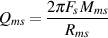 | (6.38) |
where Qms is the mechanical Q of the driver at Fs
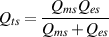 | (6.39) |
where Qts is the total Q of the driver at Fs
 | (6.40) |
where Vas is the volume of air in cubic metres which, when acted upon by a piston of
area Sd, has the same compliance as the driver’s suspension. To get Vas in litres, multiply
the result of Equation 6.40 below by 1000.
Note that ρ is the density of air (see Section ??) (1.184 kg/m3 at 25∘C), and c is the
speed of sound (346.3 m/s at 25∘C).
Large Signal Parameters
- Xmax is the maximum linear peak (or sometimes peak-to-peak) excursion (in
mm) of the cone
- Xmech is the maximum physical excursion of the driver before damage
- Pe is the thermal capacity of the driver, in watts
- Vd is the peak displacement volume, calculated by Vd = SdXmax
Other Parameters
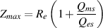 | (6.41) |
where Zmax is the impedance of the loudspeaker at Fs, used when measuring Qes and
Qms.
 | (6.42) |
where EBP is the Efficiency Bandwidth Product, an indicator of whether a driver
should be in a vented or sealed enclosure.
Znom - The nominal impedance of the loudspeaker, typically 4, 8 or 16 Ω.
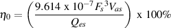 | (6.43) |
where η0 is the reference or ”power available” efficiency of the driver, in
percent.
6.9.5 Distortion and Klippel
6.9.6 Suggested Reading List
6.10 Loudspeaker acoustics
If you’re going to build a loudspeaker, one of the many things you have to consider is the
acoustical properties of the system irrespective of the electroacoustical issues. For
example, does a loudspeaker that looks like a rectangular box have a different behaviour
than one that has smoothed corners, or looks like a sphere? What is the relationship
between the radiation of the loudspeaker and the size of the drivers if you’re sitting in the
wrong place?
In this chapter, we’ll just deal with a couple of the basic issues that you have to think
about if you’re going to build a loudspeaker – or even if you’re just going to complain
about someone else’s...
6.10.1 Driver directivity
Let’s start with a very simple system. We’ll take two infinitely small loudspeakers and
place them a small distance apart from each other as is shown in Figure 6.187. We’ll
connect the two loudspeakers to a single sinusoidal signal generator so that they’re
producing the same signal at exactly the same time. We saw, once upon a time, way back
in Section 3.1.16, that if we’re standing a decent distance away from the loudspeakers,
and if we simplify things a little, then what we hear (or what a microphone
will measure) is the sum of their pressure outputs. However, that sum must
take into account the phase difference of the two loudspeaker signals at the
listening position. That phase difference is the result of the two loudspeakers being
two different distances from you (unless you’re directly in front of them, of
course...)
If you’re in a location where the two loudspeakers are the same distance from you,
then the two signals are in phase all the time, and they add together, just as we saw
back in Section 3.1.16. This is not very interesting... It’s the same signal, but
louder.
So, let’s move to one side a little, so that one of the loudspeakers is closer than the
other and think about what happens...
If we produce a low frequency (let’s say that it’s so low that the wavelength is much
greater than 2 times the distance between the loudspeakers), then the delay difference
caused by the difference in distance to the loudspeakers is small relative to the period of
the sinusoid that we’re producing. This, in turn, means that the phase difference between
the loudspeakers’ signals at the listening position is close to 0∘, so the signals add
together almost as well as if you were standing right in front of them. This is shown in
Figure 6.187.
If we now start to increase the frequency of the tone generator, the delay difference
between the loudspeakers at the listening position remains constant, but it becomes more
and more significant in proportion to the period of the signal (which is getting shorter
and shorter as the frequency goes up).
Eventually, we’ll get to a frequency where the wavelength of the sinusoid is two
times the difference in the distance to the two loudspeakers when measured from
the listening position. For example, if one loudspeaker is 20 cm closer to you
than the other, then we’re talking about a sinusoid with a wavelength of 40 cm
which corresponds to a frequency of 850 Hz (assuming a speed of sound of 340
m/s).
At this particular frequency, the signals from the two loudspeakers at the listening
position will be 180∘ out-of-phase with each other, causing the same effect as if they
were opposite in polarity – they cancel each other. In our temporarily perfect world with
omnidirectional, infinitely small loudspeakers, and no reflections from other objects, they
cancel each other completely, and you hear none of the signal at the listening position.
This is illustrated in Figure 6.188.
Note that, as the signal’s frequency went from 0 Hz up to the frequency where it first
results in complete cancellation, the phase difference of the two signals at the listening
position is moving from 0∘ to 180∘. Consequently, the level at the listening position
smoothly drops as you increase the frequency – however, we’ll be more specific about
this later.
Now let’s start at the frequency where we get complete cancellation at the listening
position and start raising the frequency once more. As before, the delay difference
between the loudspeakers’ signals is constant, but it’s increasing in proportion to the
period of the signal because the period is getting shorter. Eventually, we’ll get to a
frequency where the delay difference is equal to the period of the signal. At this point,
the difference in distance to the loudspeakers from the listening position is the same as
the wavelength of the signal they are producing. Consequently there is a 360∘ phase
difference between the two signals as is illustrated in Figure 6.189. Since we already
know that a 360∘ phase shift is identical to a 0∘ phase shift (in other words, no phase
shift) then we get complete constructive interference once again, and we hear a sine
tone with the same level as our very very low frequency tone that we started
with.
Radiation patterns – Two Loudspeaker Drivers
In the previous section, we were staying in the same listening position and changing the
frequency of the signal sent to the two infinitely small, perfectly omnidirectional
loudspeakers to see how the resulting combined signal would behave at one location.
Instead of maintaining position and changing the frequency (and ultimately resulting in a
frequency response measurement for that position), we could do the opposite – we’ll
keep the frequency constant and move our position.
In this case, we’ll maintain a constant distance from a point that is exactly in the
middle of the two loudspeakers and rotate around them, changing our angle to the
pair, but maintaining a constant distance. Note that we’re keeping a constant
distance to the pair, but the individual distances to each driver will change with the
angle.
Also, for this section, we’re going to start getting a little more specific about what
frequency we’re looking at, and what the spacing between the loudspeakers
is. Finally, we’ll assume for this entire section that the speed of sound in air
is 340 m/s, which is close enough – it might even be true, depending on the
temperature.
10 Hz
Let’s put the loudspeakers 34 cm apart and set the frequency of the tone generator to
10 Hz. The wavelength of a 10 Hz sinusoid is 34 m which 100 times longer than the
spacing between our loudspeakers. In a best-case scenario, when you’re the same
distance from two drivers, the phase difference at the listening position will be 0∘. Let’s
call the output that you measure at that location our reference level, so, on a
linear scale, we’ll arbitrarily say that this is a value of 1, which we’ll call our
reference value of 0 dB. The actual level isn’t so exciting, since it’s affected
by the power output of the loudspeakers and your distance to them. What’s
more interesting for us right now is how the level changes when your position
changes, so we’ll just compare the level at other locations to the one at the
front.
In a worst-case situation, you are standing 90∘ off-axis to the pair – in other words,
you are to one side of the loudspeaker array, so the difference in distance is as big as it
can be. In this case, the difference in distance between the speakers is 1/100th of the
wavelength of the sinusoid, which means that the phase difference at the listening
position will be 1/100th of 360∘, or 3.6∘. Since this phase difference is so small, you’ll
get almost no loss of signal to the side of the loudspeaker array compared to directly in
front of it.
If we calculate the combined output for the two loudspeakers for all angles in front of
the pair, we can plot the resulting level (since they’re omnidirectional, the back of the
pair will be symmetrical to the front, so plotting it is redundant). This is shown in Figure
6.190.
Figure 6.190 shows the output, plotted on a linear and a decibel scale, on a cartesian
plot. This is useful, but a more intuitive representation is a polar plot which shows the
angle to the loudspeaker pair as an angle on the plot rather than as the X-axis. This polar
plot can show the level on a linear scale, as is shown in Figure 6.191 or on a decibel scale
as in Figure 6.192.
At this point, you may be wondering why I’m plotting the same data on cartesian and
polar plots, both in linear and decibel scales. At the moment, I’ll admit that there’s no
good reason, but there will be later in the section.
250 Hz
Let’s now increase the frequency of the tone generator to 250 Hz, keeping the
loudspeakers in the same locations, and keeping your distance to the pair. In this particular
situation the wavelength of the tone is 4 times the separation of the loudspeaker drivers,
so if we move our listening position from 0∘ (in front) to 90∘ (to one side) of the
loudspeaker array, we’ll be changing smoothly from perfect constructive interference to a
level equivalent to what we would have gotten if only one of the loudspeakers was
playing.
If we plot the resulting output vs. angle of the listening position relative to the
loudspeaker pair for 250 Hz, we’ll get responses as are shown in Figures 6.193, 6.194
and 6.195.
Note in these plots that the signal drops from 0 dB at the front of the pair to -6 dB at
the side of the pair.
500 Hz
If we repeat the same measurements at 500 Hz, we’ll now see that as we approach
the side of the loudspeaker pair, the combined output at the listening position goes to 0,
or -∞ dB. This is because the 34 cm distance between the loudspeakers is equal to one
half the wavelength of 500 Hz. So, at the listening position, the signals are 180∘
out-of-phase, so they cancel each other completely.
If we look at the representation of the pattern on a linear polar scale, we can see
that the radiation of the loudspeaker array has what is called a lobe. This is
a teardrop-shaped area on a polar plot that tells us there is a range of angles
relative to the loudspeaker pair where the combined signal is higher than in other
places.
When the polar plot is shown on a decibel scale, the lobe appears to be much wider.
This is because a decibel scale gives us a better representation of lower-level signals, so it
appears to emphasise the quieter areas of the lobe. In fact, although many books will
show the radiation pattern of a loudspeaker on a polar plot with a linear scale as in
6.197, it makes more sense to us humans to look at the decibel version as is
shown in Figure 6.198. (However, I’ll talk later about cases where this is not
true.)
1000 Hz
When the signal has a frequency of 1 kHz, its wavelength is the same as the distance
between the loudspeakers. Consequently, we’ll get a cancellation at 30∘ off-axis to the
pair, and we’ll get complete constructive interference at 90∘. This is shown in Figures
6.199, 6.200 and 6.201.
You can see in Figures 6.200 and 6.201 that, if we’re only thinking about the “front”
of the loudspeaker pair, there are three lobes where we get a maximum output from the
array. In fact, since the back side of our pair of omnidirectional loudspeakers is
symmetrical to the front, at 1 kHz, we actually have 4 lobes in a cloverleaf-shaped
pattern.
2000 Hz
If the frequency of the tone is increased, we’ll see more and more lobes appearing.
To illustrate this, we’ll look at two more frequencies. Figures 6.202, 6.203 and 6.204
show the radiation pattern of the loudspeaker pair for 2 kHz. As you can see, this results
in 5 lobes in front of the pair.
10000 Hz
At 10 kHz, the wavelength is very small compared with the separation between the
loudspeakers, so we get a large number of lobes in front of our loudspeaker pair as can be
seen in Figures 6.205, 6.206 and 6.207.
Polar plots – More Loudspeaker Drivers
Let’s set the frequency of the signal generator to 5 kHz. We’ll leave the separation of our
infinitely small, omnidirectional loudspeakers at 34 cm and do the same measurement
of the output level relative to angle to the listening position the linear-scale
polar representation of the radiation pattern of this array is shown in Figure
6.208.
Now we’ll add an extra loudspeaker at the exact midpoint between them. So, now we
have three loudspeakers all connected in parallel to the tone generator, and we’ll repeat
our measurement.
Let’s start by looking at the cartesian representation of the result as is shown in
Figure 6.209.
There are three important things to notice in this plot.
The first, and most obvious, is the change in the relative levels of the lobes. In Figure
6.209 (with only 2 loudspeakers) we saw that there are 11 lobes, all with the same
maximum level. In Figure 6.210 (3 loudspeakers) we have the same number of lobes, but
6 of them (every alternate one) have a lower level.
The second is a question of cancellation. In the case of two loudspeakers, in between
each lobe, there is complete cancellation. On a linear cartesian plot, this means that the
dip between each bump bottoms out at a value of 0. On a dB scale, it means that
the troughs are deep notches that drop to -∞. In the case of 3 loudspeakers,
things are a little more complicated as can be seen in the dB scale plot in Figure
6.209.
Finally, there is the question of polarity. In the case of two loudspeakers, all of
our linear values ranged between 0 and 1, inclusive. However, now that we’ve
added an extra loudspeaker, if you look carefully, you’ll see that our dips in the
response on the linear scale drop below 0. This means that, at some specific angles,
the signal will be opposite in polarity to other angles. It’s counterintuitive to
represent this on a polar plot because it will look like the lobe is pointing in the
wrong direction. (This is because a negative value at 0∘ is plotted like a positive
value at 180∘. Negative values at 45∘ look like positive ones at 225∘, and so
on.)
If we increase the number to 4, equally spaced loudspeakers, with the most distant
ones staying at 34 cm, we’ll see another change in the overall radiation pattern of the
combined output at different angles. I’ll just plot the theoretical response here without
discussing it.
One thing worth mentioning here before things get more difficult to see is that the
angles of the maximum points of each lobe aren’t changing as we add more loudspeakers
– This is determined by the separation between the two outside loudspeakers.
The only things that are really changing are the individual amplitudes of the
lobes.
Let’s now increase to 8 drivers. Now we can see in Figures 6.215, 6.216, and 6.217
we now have one principal lobe that beams at an angle of 0∘. All other lobes are much
lower in level.
If we double the number of loudspeakers again, to a total of 16, we’ll see that the
difference between the main lobe and all of the others becomes greater as is shown in
Figures 6.218, 6.219, and 6.220.
Let’s go crazy. We’ll put a very large number of loudspeakers – 256, equally spaced
units in a straight line, with the outside ones still 24 cm apart. (In other words, we have
less than 1 mm between each loudspeaker.) If we plot the theoretical radiation pattern of
this array, we’ll see that there is basically just one main beam at 5 kHz as is shown in
Figures 6.221, 6.222, and 6.223.
Polar plots – A Driver simplified to a Piston
Up to now, we’ve been looking at a weird sort of thing... a collection of infinitely-small,
omnidirectional loudspeakers, sitting in a row. This, of course, doesn’t exist in real life,
however, it’s a good way to think of all the molecules sitting next to each other on the
face of a loudspeaker.
That which we call a “loudspeaker driver” in real life is usually more like a cone with
a bump at the bottom, as we saw an earlier section. Let’s simplify that shape and pretend
that it’s just a flat circle that moves in and out its cabinet. We’ll also simplify the border
between the driver and the cabinet it sits in and say that there is no connection
between the two, but there’s no leak either. Also, we’ll pretend that the face of
the speaker cabinet is infinitely big. So, we have a wall that extends to infinity
in all directions (what loudspeaker engineers call a “2 π baffle” (say “two-pi
baffle”)), and there’s a hole in that wall with a circular piston that moves in and
out.
Let’s pretend that we did have such a thing and we took a look at its directivity.
As we’ve already seen with the array of drivers, we’d expect our “speaker”
(actually, a piston) to be omnidirectional at low frequencies and increasingly
directional as we go up in frequency. It probably won’t come as a surprise to
find out that this is exactly what happens. Figures 6.224 and 6.225 show the
output of a piston with a diameter of 34 cm at frequencies ranging from 10 Hz
to 10 kHz, with an angular range of ±90∘. You can see there that we get an
omnidirectional response at low frequencies, and a very narrow beam off the front of
the piston at high frequencies. The frequency area where we transition from
omni to directional is around the frequency that has a wavelength equal to the
diameter of the piston – 1 kHz (plus/minus an octave... it’s a wide transition
band...).
You can also see in Figure 6.224, just like in the case of the array, that, at some
angles at higher frequencies, the signal is opposite in polarity from the main on-axis
beam.
If we plot the same information in decibels, we get the graphs in Figures
6.226 and 6.227. Notice that, at 10 kHz, we’re more than 20 dB down from the
level on-axis, at less than 10∘ off-axis. This means, in real life, that if you move
just a little bit out of that beam, all of your high-end will seem to completely
disappear...
Let’s consider this in a different way. All of the plots in this section so far show you
what happens if you play a frequency, and then move out of the direct line of fire.
What’s more likely is that you’re listening to more than one frequency – music,
for example, and sitting somewhere off-axis. So, let’s look at the frequency
response of the piston at different angles. This is shown in Figures 6.228, 6.229
and 6.230. You should see in these plots that, as you sit further off-axis to the
loudspeaker (i.e. the more to the side) the lower the high-frequency cutoff of the
signal.
Okay, so by now, you’re probably sitting there thinking “this is lovely, but he’s only
talking about theoretical things like infinitely small speakers or flat-faced pistons... what
about real loudspeakers?” Well... I have some very bad news... I’m not going to talk
about real loudspeakers. The reason for this glaring omission is that the actual
shape of a loudspeaker driver has a huge effect on the details of directional
characteristics, but without getting into some very serious math that goes way
over my head, we won’t get anywhere. So, this is as close as I’m going to get
to the Truth. If you want to come closer, then you’ll just have to go looking
somewhere else... (John Eargle’s Loudspeaker Handbook is a good choice)
Sorry.
So what?
There are a number of reasons why you should care about this.
The simplest reason is knowing the relationship between the diameter of a
loudspeaker, its frequency range, and the resulting range of movement you
have. If you have a 34 cm diameter woofer that is running up to 10 kHz (this is
silly...) then you have to be in the on-axis beam, or you won’t hear any high
end.
START WRITING HERE!!
6.10.2 Enclosures
- Enclosure Design (i.e. “what does the box look like?”) of which there are a number of
possibilities including the following:
- Dipole Radiator (no enclosure) - Infinite Baffle - Finite Baffle - Folded
Baffle - Sealed Cabinet (aka Acoustic Suspension) - Ported Cabinet (aka Bass
Reflex)
- Horns (aka Compression Driver)
Dipole Radiator
(no enclosure)
aka a Doublet Radiator
Since both sides of a dipole radiator’s diaphragm are exposed to the outside world
(better known as your listening room) there are opposite polarity pressures being
generated in the same space (albeit at different locations) simultaneously. As the
diaphragm moves “outwards” (i.e. towards the listener), the resulting air pressure at the
“front” of the diaphragm is positive while the pressure at the back of the diaphragm is of
equal magnitude but opposite polarity.
At high frequencies, the diaphragm beams (meaning that it’s directional
– it only sends the energy out in a narrow beam rather than dispersing it in
all directions) as if the rear side of the diaphragm were sealed. The result of
this is that the negative pressure generated by the rear of the diaphragm does
not reach the listener. For more information on beaming see section 1.6 of the
Loudspeaker and Headphone Handbook edited by John Borwick and published by
Butterworth.
At low frequencies, the delay time required for energy to travel from the back of the
diaphragm to the front and towards the listener is a negligible part of the phase of the
wave (i.e. the distance around the diaphragm is very small compared to the
wavelength of the frequency). Since the energy at the rear of the diaphragm is
opposite in polarity to the front, the two cancel each other out at the listening
position.
The result of all this is that a dipole radiator doesn’t have a very good low frequency
response – in fact, it acts much like a high pass filter with a slope of 6 dB/octave
and a cutoff frequency which is dependent on the physical dimensions of the
diaphragm.
How do we fix this?
Infinite Baffle
The biggest problem with a dipole radiator is caused by the fact that the energy from the
rear of the diaphragm reaches the listener at the front of the diaphragm. The simplest
solution to this issue is to seal the back of the diaphragm as shown.
This is called an “infinite baffle” because the diaphragm is essentially mounted on a
wall of infinite dimensions. (Another way to draw this would have been to put the
diaphragm mounted in a small hole in a wall that goes out forever. The problem with
that kind of drawing is that my stick man wouldn’t have had anything to stand
on.)
Disadvantages
- You’re automatically throwing away half of your energy (the half that’s radiated by
the rear of the diaphragm
- Costs... How do you build a wall of infinite dimensions?
Advantages
- Lower low-frequency cutoff than a dipole radiator.
Now the low cutoff frequency is dependent on the diameter of the diaphragm
according to the following equation:
 | (6.44) |
Where fc is the low frequency cutoff in Hz (-3 dB point)
c is the speed of sound in air in m/s
D is the diameter of the loudspeaker in m
Unlike the dipole radiator, frequencies below the cutoff have a pressure
response of 12 dB/octave (instead of 6 dB/octave). Therefore, if we’re going down
in frequency comparing a dipole radiator and an infinite baffle with identical
diaphragms, the infinite baffle will go lower, but drops off more quickly past that
frequency.
Finite Baffle
Instead of trying to build a baffle with infinite dimensions, what would happen if
we mounted the diaphragm on a circular baffle of finite dimensions as shown
below?
Now, the circular baffle causes the energy from the rear of the driver to reach the
listener with a given delay time determined by the dimensions of the baffle. This causes a
comb-filtering effect with the first notch happening where the path length from
the rear of the driver to the front of the baffle equals one wavelength as shown
below:
One solution to this problem is to create multiple path lengths by using an
irregularly-shaped baffle. This causes multiple delay times for the pressure from the rear
of the diaphragm to reach the front of the baffle. The technique will eliminate the comb
filtering effect (no notches above the transition frequency) but we still have a 6 dB/octave
slope in the low end (below the transition frequency). If the baffle is very big
(approaching infinite relative to the wavelength of the lowest frequencies) then the slop
in the low end approaches 12 dB/octave – essentially, we have the same effect as if it
were an infinite baffle.
If the resonant frequency of the driver, below which the roll-off occurs at a slope of 6
dB/octave, is the same as (or close to) the transition frequency of the baffle, the slope
becomes 12 or 18 dB/octave (dependent on the size of the baffle – the slopes add). The
resonant frequency of the driver is the rate at which the driver would oscillate if your
thumped it with your finger – though we’ll talk about that a little more in the section on
impedance.
What do you do if you don’t have enough room in your home for big baffles? You
fold them up!
Folded Baffle
(aka Open-back Cabinet)
A folded baffle is essentially a large flat baffle that has been “folded” into a tube
which is open on one end (the back) and sealed by the driver at the other end as is shown
below.
The fact that there’s a half-open tube in the picture causes a nasty resonance (see the
section on resonance in the Acoustics section of this textbook for more info on why this
happens) at a frequency determined by the length of the tube.
wavelength of the resonant frequency = 4 * length of the tube
The low frequency response of this system is the same as in the case of finite
baffles.
Sealed Cabinet
(aka Acoustic Suspension)
We can eliminate the resonance of an open-back cabinet by sealing it up, thus turning
the tube into a box.
Now the air sealed inside the enclosure acts as a spring which pushes back against
the rear of the diaphragm. This has a number of subsequent effects:
- increased resonant frequency of the driver
- reduced efficiency of the driver (because it has to push and pull the “spring” in
addition to the air in the room)
- non-symmetrical distortion (because pushing in on the “spring” has a different
response than pulling out on it)
We’re throwing away a lot of energy as in the case of the infinite baffle because the
back of the driver is sealed off to the world.
Usually the enclosure has an acoustic resonant frequency (sort of like little room
modes) which is lower than the (now raised...) resonant frequency of the driver. This
effectively lowers the low cutoff frequency of the entire system, below which the slope is
typically 12 dB/octave.
Ported Cabinet
(aka Bass Reflex)
You can achieve a lower low cutoff frequency in a sealed cabinet if you cut a hole in
it – the location is up to you (although, obviously, different locations will have different
effects...)
If you match the cabinet resonance, which is determined by the volume of the cabinet
and the diameter and length of the hole (look up Helmholtz resonators in the Acoustics
section), with the speaker driver resonance properly (NOTE: Could someone explain to
me what a “properly matched” cabinet and driver resonance means?), you can get a lower
low frequency cutoff than a sealed cabinet, but the low frequencies now roll off at a slope
of 24 dB/octave.
Horns
(aka Compression Drivers)
The efficiency of a system in transferring power is determined by how the power
delivered to the system relates to the power received in the room. For example, if I were
to send a signal to a resistor from a function generator with an output impedance of 50Ω,
I would get the most power dissipation in the resistor if it had a value of 50Ω. Any other
value would mean that less power would be dissipated by the device. This is
because its impedance would be matched to the internal impedance of the function
generator.
Consider loudspeakers to have the same problem: the transfer motion (kinetic energy,
if you’re a geek) or power from a moving diaphragm to the air surrounding it.
The problem is that the air has much lower acoustic impedance than the driver
(meaning, it’s easier to move back and forth), therefore our system isn’t very
efficient.
Just as we could use a transformer to match electrical impedances in a circuit
(providing a Req rather than the actual R) we can use something called a horn to match
the acoustic impedances between a driver and the air.
There are a couple of things to point out regarding this approach:
- The diaphragm is mounted in a small chamber which opens to the horn
- At point “a” (the small area of the horn) there is a small area of air undergoing a
large excursion. The purpose of the horn is to slowly change this into the energy at point
“b” where we have a large area with a small excursion. In other words, the horn acts as
an impedance matching device, ensuring that we have an optimal power transfer from the
diaphragm to the air in the room.
- Notice that the diaphragm is large relative to the opening to the horn. This means
that, if the diaphragm moves as a single unit (which it effectively does) there is a phase
difference (caused by propagation delay differences to the horn) between the pressure
caused by the centre of the diaphragm and the pressure caused by the edge of the
diaphragm. Luckily, this problem can be avoided with the insertion of a plug which
ensures that the path lengths from different parts of the diaphragm to the centre of the
throat fo the horn are all equal.
In the above diagram, the large black area is the cross section of the plug with hole
drilled in it (the white lines). Each hole is the same length, ensuring that there is no
interference, either constructive or destructive, caused by multiple path lengths from the
diaphragm to the horn.
6.10.3 Other Issues
Beaming
As a general rule of thumb, a loudspeaker is almost completely omnidirectional (it
radiates energy spherically – in all directions) when the driver is equal to or less than 1/4
the wavelength of the frequency being produced. The higher the frequency, the more
directional the driver.
Why is this a problem?
High frequencies are very directional, therefore if your ear is not in the direct “line of
fire” of the speaker (that is to say, “on axis”) then you are getting some high-frequency
roll-off.
In the case of low frequencies, the loudspeaker is omnidirectional, therefore you are
getting energy radiating behind and to the sides of the speaker. If there’s a nearby wall,
floor or ceiling, the pressure which bounces off it will add to that which is radiating
forward and you’ll get a boost in the low end.
- If you’re near 1 surface, you get 3 dB more power in the low end
- If you’re near 2 surfaces, you get 6 dB more power in the low end
- If you’re near 3 surfaces, you get 9 dB more power in the low end
The moral of this story? Unless you want more low end, don’t put your loudspeaker
in the corner of the room.
Multiple drivers
We said much earlier that drivers are usually optimized for specific frequency bands.
Therefore, an easy way to get a wide-band loudspeaker is to use multiple drivers to cover
the entire audio range. Most commonly seen these days are 2-way loudspeakers
(meaning 2 drivers, usually in 1 enclosure), although there are many variations on
this.
If you’re going to use multiple drivers, then you have some issues to contend
with:
1 – Crossovers
- You don’t want to send high frequencies to a low frequency driver (aka woofer or
low frequencies to a high-frequency driver (aka tweeter). In order to avoid this, you filter
the signals getting sent to each driver – the woofer’s signal is routed through a low-pass
filter, while the tweeter’s is filtered using a high-pass. If you are using mid-range drivers
as well, then you use a band-pass filter for the signal. This combination of filters is
known as a crossover.
Most filters in crossovers have slopes of 12 or 18 dB/octave (although it’s not
uncommon to see steeper slopes) and have very specific designs to minimize phase
distortion around the crossover frequencies (the frequencies where the two filters overlap
and therefore the two drivers are producing roughly equal energy) This is particularly
important because crossover frequencies are frequently (sorry... I couldn’t resist at
least one pun) around the 1 – 3 kHz range – the most sensitive band of our
hearing.
There are two basic types of crossovers, active and passive.
Passive crossovers
These are probably what you have in your home. Your power amplifier sends a
full-bandwidth signal to the crossover in the loudspeaker enclosure which, in turn, sends
filtered signals to the various drivers. This system has a drawback in that it wastes power
from your amplifier – anything that is filtered out is lost power. “Audiophiles”
(translation: “people with too much disposable income who spend more time reading
reviews of their audio equipment than they do actually listening to it”) also
complain about issues like back EMF and cabinet vibrations which may or may
not affect the crossover. (I’ll believe this when I see some data on it...). The
advantage of passive crossovers is that they’re idiot-proof. You plug in one
amplifier to one speaker input and the system works and works well. Also – they’re
inexpensive.
Active crossovers
These are filters that precede the power amplifier in the audio chain (the amplifier is then
directly connected to the individual driver). They are more efficient, since you only
amplify the required frequency band for each driver – then again, they’re more expensive
because you have to buy the crossover plus extra amplifiers.
2 – Crossover Distortion
There is a band of frequencies around the cutoffs of the crossover filters where the
drivers overlap. At this point you have roughly equal energy being emitted by at
least two diaphragms. There is an acoustic interaction between these two which
must be considered, particularly because it is in the middle of the audio range
usually.
In order to minimize problems in this band, the drivers must have matched distances
to the listener, otherwise, you’ll get comb filtering due to propagation delay differences.
This so-called time aligning can be done in one of two ways. You can either build the
enclosure such that the tweeter is set back into the face of the cabinet, so its voice coil is
vertically aligned with the voice coil of the deeper woofer. Or, alternately you can use an
electronic delay to retard the arrival of the signal at the closer driver by an appropriate
amount.
3 – Interaction between drivers
Remember that the air inside the enclosure acts like a spring which pushes and pulls
the drivers contrary to the direction you want them to move in. Imagine a woofer
moving into a cabinet. This increases the air pressure inside the enclosure which
pushes out against both the woofer AND the tweeter. This is bad thing. Some
manufacturers get around this problem by putting divided sections inside the cabinet –
others simply build separate cabinets – one for each driver (as in the B and W
801).
6.10.4 Loudspeaker driver non-linearities
Until I get something written on this topic, I would highly recommend that you
just read anything you can by Wolfgang Klippel. His tutorials on loudspeaker
nonlinearities are available from the Audio Engineering Society and his own
website.
Suggested Reading List