2.1.1 Introduction
Everything, everywhere is made of molecules, which in turn are made of atoms (except
in the case of the elements in which the molecules are atoms). Atoms can be
thought of as being made of two things, electrons that orbit a nucleus. The nucleus
is made of protons and neutrons. Each of these three particles (the electrons,
neutrons and protons) has a specific charge or electrical capacity. (Apparently,
charge is a difficult thing to define. One way to think of it is that charge is the
electrical equivalent of magnetism - it is the ability of a sub-atomic particle (for
example, an electron) to be attracted to (or repelled by) another sub-atomic particle.
Since atoms are made of sub-atomic particles, and everything is made of atoms,
then some materials (like balloons) are able to hold a charge and be attracted to
other materials (like ceilings).) Electrons have a negative charge, protons have a
positive charge, and neutrons have no charge. As a result, the electrons, which
orbit around the nucleus like planets around the sun, don’t go flying off into
the next atom because their negative charge attracts to the positive charge of
the protons. Just as gravity ensures that the planets keep orbiting around the
sun and don’t go flying off into space, charge keeps the electrons orbiting the
nucleus.
There is a slight difference between the orbits of the planets and the orbits of the
electrons. In the case of the solar system, every planet maintains a unique orbit – each being
a different distance from the sun, forming roughly concentric ellipses from Mercury out to
Pluto
(or sometimes Neptune). In an atom, the electrons group together into what are called
valence shells. A valence shell is much like an orbit that is shared by a number of
electrons. Different valence shells have different numbers of electrons that, together, all
add up to the total number in the atom. Different atoms have a different number of
electrons, depending on the substance. This number can be found up in a periodic table
of the elements, a simple version of which is shown in Figure 2.1. For example, the
element hydrogen, which is number 1 on the periodic table, has 1 electron in
each of its atoms; copper, on the other hand, is number 29 and therefore has 29
electrons.
Each valence shell likes to have a specific number of electrons in it to be stable. The
inside shell is “full” when it has 2 electrons. The number of electrons required in each
shell outside that one is a little complicated but is well-explained in any high-school
chemistry textbook.
Let’s look at a diagram of two atoms. As can be seen in the helium atom in Figure
2.2, all of the valence shells are full, the copper atom, on the other hand, has just one
lonely electron in its outermost shell. This difference between the two atom structures
give the two substances very different characteristics.
In the case of the helium atom, since all the valence shells are full, the atom is very
stable. The nucleus holds on to its electrons very tightly and will not let go
without a great deal of persuasion, nor will it accept any new stray electrons. The
copper atom, in comparison, has weakly-held electron that can be nudged out of
place. The questions are, how does one “nudge” an electron, and where does it
go when released? The answers are rather simple: we push the electron out
of the atom with another electron from an adjacent atom. The new electron
takes its place and the now-free particle moves to the next atom to push out its
electron.
So essentially, if we have a wire made of a long string of copper atoms, and we add
some electrons to one end of it, and give the electrons on the other end somewhere to go,
then we can have a flow of particles through the metal.
2.1.2 Current and EMF (Voltage)
I used to have a slight plumbing problem in my kitchen. I had two sinks, side by side, one
for washing dishes and one for putting the washed dishes in to dry. The drain of the two
sinks fed into a single drain which has built up some rust inside over the years (I lived in
an old building).
When I filled up one sink with water and pulled the plug, the water goes down the
drain, but can’t get down through the bottom drain as quickly as it should, so the result is
that my second sink fills up with water coming up through its drain from the other
sink.
Why does this happen? Well – the first answer is “gravity” – but there’s more to it
than that. Think of the two sinks as two tanks joined by a pipe at their bottoms. We’ll put
different amounts of water in each sink.
The water in the sink on the left weighs a lot – you can prove this by trying to lift the
tank. So, the water is pushing down on the tank – but we also have to consider that
the water at the top of the tank is pushing down on the water at the bottom.
Thus there is more water pressure at the bottom than the top. Think of it as the
molecules being squeezed together at the bottom of the tank – a result of the
weight of all the water above it. Since there’s more water in the tank on the left,
there is more pressure at the bottom of the left tank than there is in the right
tank.
Now consider the pipe. On the left end, we have the water pressure trying to push the
water through the pipe, on the right end, we also have pressure pushing against the water,
but less so than on the left. The result is that the water flows through the pipe from left to
right. This continues until the pressure at both ends of the pipe is the same – or, we have
the same water level in each tank.
We also have to think about how much water flows through the pipe in a given
amount of time. If the difference in water pressure between the two ends is quite high,
then the water will flow quite quickly though the pipe. If the difference in pressure is
small, then only a small amount of water will flow. Thus the flow of the water (the
volume which passes a point in the pipe per amount of time) is proportional on
the pressure difference. If the pressure difference goes up, then the flow goes
up.
The same can be said of electricity, or the flow of electrons through a wire. If we
connect two “tanks” of electrons, one at either end of the wire, and one “tank” has
more electrons (or more pressure) than the other, then the electrons will flow
through the wire, bumping from atom to atom, until the two tanks reach the same
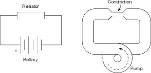
level. Normally we call the two tanks a battery. Batteries have two terminals –
one is the opening to a tank full of too many electrons (the negative terminal –
because electrons are negative) and the other the opening to a tank with too
few electrons (the positive terminal). If we connect a wire between the two
terminals (don’t try this at home!) then the surplus electrons at the negative
terminal will flow through to the positive terminal until the two terminals have the
same number of electrons in them. The number of surplus electrons in the tank
determines the “pressure” or voltage (abbreviated V and measured in volts)
being put on the terminal. (Note: once upon a time, people used to call this
electromotive force or EMF but as knowledge increases from generation to
generation, so does laziness, apparently... So, most people today call it voltage
instead of EMF. Never one to go against the mob, I’ll do the same.) The more
electrons, the more voltage, or electrical pressure. The flow of electrons in the
wire is called current (abbreviated I and measured in amperes or amps) and is
actually a specific number of electrons passing a point in the wire every second
(6.24150948?1018 or 6,241,509,480,000,000,000 to be precise – possibly even
accurate...) .
(Note: some people call this “amperage” – but it’s not common enough to be a standard...
yet...) If we increase the voltage (pressure) difference between the two ends of the wire,
then the current (flow) will increase, just as the water in our pipe between the two
tanks.
There’s one important point to remember when you’re talking about current. Due to a
bad guess on the part of Benjamin Franklin, current flows in the opposite direction to the
electrons in the wire, so while the electrons are flowing from the negative to the positive
terminal, the current is flowing from positive to negative. This system is called
conventional current theory. There are some books out there that follow the flow of
electrons – and therefore say that current flows from negative to positive. It
really doesn’t matter which system you’re using, so long as you know which is
which.
Let’s now replace the two tanks by a pump with pipe connecting its output to its input
– that way, we won’t run out of water. When the pump is turned on, it decreases the
water pressure at its input in order to increase the pressure at its output. The
water in the pipe doesn’t enjoy having different pressures at different points
in the same pipe so it tries to equalize by moving some water molecules out
of the high pressure area and into the low pressure area. This creates water
flow through the pipe, and the process continues until the pump is switched
off.
2.1.3 Resistance and Ohm’s Law
Let’s complicate matters a little by putting a constriction in the pipe – a small section
where the diameter of the tube is narrower than anywhere else in the system. If we keep
the same pressure difference created by the pump, then less water will go through
because of the restriction – therefore, in order to get the same amount of water through
the pipe as before, we’ll have to increase the pressure difference. So the higher the
pressure difference, the higher the flow; the greater the restriction, the smaller the
flow.
We’ll also have a situation where the pressure at the input to the restriction is
different than that at the output. This is because the water molecules are bunching up at
the point where they are trying to get through the smaller pipe. In fact the pressure at
the output of the pump will be the same as the input of the restriction while
the pressure at the input of the pump will match the output of the restriction.
We could also say that there is a drop in pressure across the smaller diameter
pipe.
We can have almost exactly the same scenario with electricity instead of water. The
electrical equivalent to the restriction is called a resistor. It’s a small component
which resists the current, or flow of electrons. If we place a resistor in the wire,
like the restriction in the pipe, we’ll reduce the current as is shown in Figure
2.3.
The higher the voltage difference, the higher the current. The bigger the resistor, the
smaller the current. Just as in the case of the water, there is a drop in voltage (electrical
“pressure”) across the resistor. The voltage at the output of the resistor is lower than that
at its input. Normally this is expressed as an equation called Ohm’s Law which goes like
this:
 | (2.1) |
or
 | (2.2) |
where V is in volts (abbreviated V), I is in amps (abbreviated A) and R is in ohms
(abbreviated Ω).
We use this equation to define how much resistance we have. The rule is that 1 V of
potential difference across a resistor will make 1 A of current flow through it if the
resistor has a value of 1 Ω. An ohm is simply a measurement of how much the flow of
electrons is resisted.
The equation is also used to calculate one component of an electrical circuit given the
other two. For example, if you know the current through and the value of a resistor, the
voltage drop across it can be calculated.
Everything resists the flow of electrons to different degrees. Copper doesn’t resist
very much at all – in other words, it conducts electricity, so it is used as wiring; rubber,
on the other hand, has a very high resistance, in fact it has an almost infinite resistance so
we call it an insulator
2.1.4 Power and Watt’s Law
If we return to the example of a pump creating flow through a pipe, it’s pretty
obvious that this little system is useless for anything other than wasting the energy
required to run the pump. If we were smart we’d put some kind of turbine or
waterwheel in the pipe which would be connected to something which does work –
any kind of work. Once upon a time a similar system was used to cut logs –
connect the waterwheel to a circular saw; nowadays we do things like connecting
generators to the turbine to generate electricity to power circular saws. In either
case, we’re using the energy or power in the moving water to do something
useful.
How can we measure or calculate how much work our waterwheel is capable of
doing? Well, there are two variables involved with which we are concerned – the pressure
behind the water and the quantity of water flowing through the pipe and turbine. If there
is more pressure, there is more energy in the water to do stuff; if there is more flow, then
there is more water to do stuff.
Electricity can be used in the same fashion – we can put a small device in the wire
between the two battery terminals which will convert the power in the electrical current
into some useful work like brewing coffee or powering an electric stapler. We have the
same equivalent components to concern us, except now they are named current and
voltage. The higher the voltage or the higher the current, the more energy in our system –
therefore the power it has.
This relationship can be expressed by an equation called Watt’s Law which is as
follows:
 | (2.3) |
or
 | (2.4) |
where P is in Watts, V is in volts and I is in amps.
Just as Ohm’s law defines the ohm, Watt’s law defines the watt to be the amount of
power consumed by a device which, when supplied with 1 volt of difference across its
terminals will use 1 amp of current.
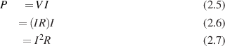
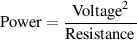
We can create a variation on Watt’s law by combining it with Ohm’s law as
follows:
P = VI and V = IR
therefore
and
Note that, as is shown in the equation above on the right, the power is proportional to
the square of the voltage. This gem of wisdom will come in handy later.
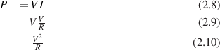
2.1.5 Alternating vs. Direct Current
So far we have been talking about a constant supply of voltage – one that doesn’t change
over time, such as a battery before it starts to run down. This is what is commonly know
of as direct current or DC which is to say that there is no change in voltage over a period
of time. This is not the kind of electricity found coming out of the sockets in your wall at
home. The electricity supplied by your electricity company changes over short periods of
time (it changes over long periods of time as well, but that’s an entirely different
story...) Every second, the voltage difference between the two terminals in your
wall socket fluctuates between about -170 V and 170 V sixty times a second (if
you live in North America, at least...). This brings up two important points to
discuss.
Firstly, the negative voltage... All a negative voltage means is that the electrons are
flowing in a direction opposite to that being measured. There are more electrons in the
tested point in the circuit than there are in the reference point, therefore more negative
charge. If you think of this in terms of the two tanks of water – if we’re sitting at the
bottom of the empty tank, and we measure the relative pressure of the full one, its
pressure will be more, and therefore positive relative to your reference. If you’re at
the bottom of the full tank and you measure the pressure at the bottom of the
empty one, you’ll find that it’s less than your reference and therefore negative.
(It’s like describing someone by their height. It doesn’t matter how tall or short
someone is – if you say they’re tall, it probably means that they’re taller than
you.)
Secondly, the idea that the voltage is fluctuating. When you plug your coffee maker
into the wall, you’ll notice that the plug has two terminals. One is a reference voltage
which stays constant (normally called a “cold” wire in this case...) and one is the
“hot” wire which changes in voltage relative to the cold wire. The device in the
coffee maker which is doing the work is connected with each of these two wires.
When the voltage in the hot wire is positive in comparison to the cold wire, the
current flows from hot through the coffee maker to cold. One one-hundred and
twentieth of a second later the hot wire is negative compared to the cold, the
current flows from cold to hot. This is commonly known as alternating current or
AC.
So remember, alternating current means that both the voltage and the current are
changing in time.
2.1.6 RMS
Look at a light bulb. Not directly – you’ll hurt your eyes – actually let’s just think of a
lightbulb. I turn on the switch on my wall and that closes a connection which sends
electricity to the bulb. That electricity flows through the bulb which is slightly
resistive. The result of the resistance in the bulb is that it has to burn off power
which it does by heating up – so much that it starts to glow. But remember,
the electricity which I’m sending to the bulb is not constant – it’s fluctuating
up and down between -170 and 170 volts. Since it takes a little while for the
bulb to heat up and cool down, its always lagging behind the voltage change –
actually, it’s so slow that it stays virtually constant in temperature and therefore
brightness.
The light bulb does not respond to instantaneous voltage values – instead, it burns off
an average amount of power over time. That average is essentially an equivalent DC
voltage that would result in the same power dissipation. The question is, how do we
calculate it?
First we’ll begin by looking at the average voltage delivered to your lightbulb by the
electricity company. If we average the voltage for the full 360∘ of the sine wave that they
provide to the outlets in your house, you’d wind up with 0 V – because the voltage is
negative as much as it’s positive in the full wave – it’s symmetrical around 0 V. This is
not a good way for the hydro company to decide on how much to bill you, because your
monthly cost would be 0 dollars. (Sounds good to me – but bad to the electricity
company...)
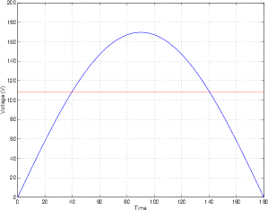
What if we only consider one half of a cycle of the 60 Hz waveform? Therefore, the
voltage curve looks like the first half of a sine wave. There are 180∘ in this section of the
wave. If we were to measure the voltage at each degree of the wave, add the results
together and divide by 180 (in other words, find the average voltage) we would come up
with a number which is 63.6% of the peak value of the wave. For example, the hydro
company gives me a 170 volt peak sine wave. Therefore, the average voltage which I
receive for the positive half of each wave is 170 V * 0.636 or 108.1 V as is shown in
Figure 2.5.
This does not, however give me the equivalent DC voltage level which would match
my AC power usage, because our calculation did not bring power into account. In
order to find this level, we have to complicate matters a little. We know from
Watt’s law and Ohm’s law that P = V2∕R. Therefore, if we have an AC wave of
170Vpeak in a circuit containing a 1Ω resistor, the peak power consumption
is
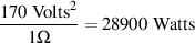 | (2.11) |
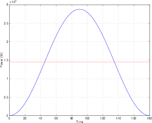
But this is the power consumption for one point in time, when the voltage level is
actually at 170 V. The rest of the time, the voltage is either swinging on its way up to 170
V or on its way down from 170 V. The power consumption curve would no longer be a
sine wave, but a sin2 wave. Think of it as taking all of those 180 voltage measurements
(one for each degree) and squaring each one. From this list of 180 numbers (the
instantaneous power consumption for each of the 180∘) we can find the average power
consumed for a half of a waveform. This number turns out to be 0.5 of the peak
power, or, in the above case, 0.5*28900 Watts, or 14450 W as is shown in Figure
2.6.
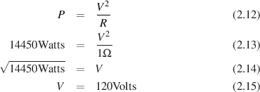
This gives us the average power consumption of the resistor, but what is the
equivalent DC voltage which would result in this consumption? We find this by using
Watt’s law in reverse as follows:
Therefore, 120 VDC would result in the same power consumption over a period of
time as a 170 VAC wave. This equivalent is called the Root Mean Square or RMS of the
AC voltage. We call it this because it’s the square root of the mean (or average) of the
square of the original voltage.
In other words, a lightbulb in a lamp plugged into the wall (remember, it’s being fed
170Vpeak AC sine wave) will be exactly as bright if it’s fed 120 VDC.
Just for a point of reference, the RMS value of a sine wave is always 0.707 of the
peak value and the RMS value of a square wave (with a 50% duty cycle) is always the
peak value. If you use other waveforms, the relationship between the peak value and the
RMS value changes.
This relationship between the RMS and the peak value of a waveform is called the
crest factor. This is a number that describes the ratio of the peak to the RMS of the
signal, therefore
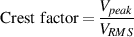 | (2.16) |
So, the crest factor of a sine wave is 1.41 (or  ). The crest factor of a square wave is
1.
). The crest factor of a square wave is
1.
This causes a small problem when you’re using a digital volt meter. The reading on
these devices ostensibly show you the RMS value of the AC waveform you’re measuring,
but they don’t really measure the RMS value. They measure the peak value of the wave,
and then multiply that value by 0.707 – therefore they’re assuming that you’re measuring
a sine wave. If the waveform is anything other than a sine, then the measurement
will be incorrect (unless you’ve thrown out a ton of money on a True RMS
multimeter...)
RMS Time Constants
There’s just one small problem with this explanation. We’re talking about an RMS value
of an alternating voltage being determined in part by an average of the instantaneous
voltages over a period of time called the time constant. In Figure 2.6, we’re assuming that
the signal is averaged for at least one half of one cycle for the sine wave. If the average is
taken for anything more than one half of a cycle, then our math will work out fine. What
if this wasn’t the case, however? What if the time constant was shorter than one half of a
cycle?
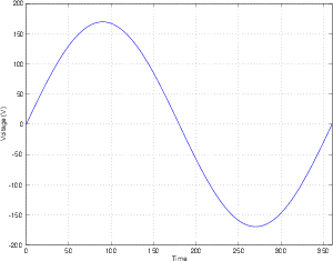
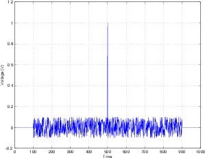
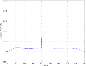
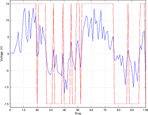
Take a look at the signal in Figure 2.7. This signal usually has a pretty low level, but
there’s a spike in the middle of it. This signal is comprised of a string of 1000 values,
numbered from 1 to 1000. If we assume that this a voltage level, then it can be converted
to a power value by squaring it (we’ll keep assuming that the resistance is 1 Ω). That
power curve is shown in Figure 2.8.
Now, let’s make a running average of the values in this signal. One way to do
this would be to take all 1000 values that are plotted in Figure 2.8 and find the
average. Instead, let’s use an average of 100 values (the length of this window in
time is our time constant). So, the first average will be the values 1 to 100. The
second average will be 2 to 101 and so on until we get to the average of values
901 to 1000. If these averages are plotted, they’ll look like the graph in Figure
2.9.
There are a couple of things to note about this signal. Firstly, notice how the signal
gradually ramps in at the beginning. This is because, as the time window that we’re using
for the average gradually “slides” over the transition from no signal to a low-level signal,
the total average gradually increases. Also notice that what was a very short,
very high level spike in the signal in the instantaneous power curve becomes a
very wide (in fact, the width of the time constant), much lower-level signal
(notice the scale of the y-axis). This is because the short spike is just getting
thrown into an average with a lot of low-level signals, so the RMS value is much
lower. Finally, the end ramps out just as the beginning ramped in for the same
reasons.
So, we can now see that the RMS value is potentially much smaller than the peak
value, but that this relationship is highly dependent on the time constant of the RMS
detection. The shorter the time constant, the closer the RMS value is to the instantaneous
peak value (in fact, if the time constant was infinitely short, then the RMS would equal
the peak...).
The moral of the story is that it’s not enough to just know that you’re being given the
RMS value, you’ll also need to know what the time constant of that RMS value
is.
2.1.7 Suggested Reading List
Fundamentals of Service: Electrical Systems, John Deere Service Publication
Basic Electricity, R. Miller
The Incredible Illustrated Electricity Book, D.R. Riso
Elements of Electricity, W.H. Timbie
Introduction to Electronic Technology, R.J. Romanek
Electricity and Basic Electronics, S.R. Matt
Electricity: Principles and Applications, R. J. Fowler
Basic Electricity: Theory and Practice, M. Kaufman and J.A. Wilson
2.2 The Decibel
Thanks to Mr. Ray Rayburn for his proofreading of and suggestions for this
section.
2.2.1 Gain
Lesson 1 for almost all recording engineers comes from the classic movie “Spinal Tap”
where we all learned that the only reason for buying any piece of audio gear is to
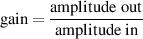
make things louder (“It goes all the way up to 11...”) The amount by which
a device makes a signal louder or quieter is called the gain of the device. If
the output of the device is two times the amplitude of the input, then we say
that the device has a gain of 2. This can be easily calculated using Equation
2.17.
 | (2.17) |
Note that you can use gain for evil as well as good - you can have a gain of
less than 1 (but more than 0) which means that the output is quieter than the
input.
If the gain equals 1, then the output is identical to the input.
If the gain is 0, then this means that the output of the device is 0, regardless of the
input.
Finally, if the device has a negative gain, then the output will have an opposite
polarity compared to the input. (As you go through this section, you should always keep
in mind that a negative gain is different from a gain with a negative value in dB... but
we’ll straighten this out as we go along.)
(Incidentally, Lesson 2 for recording engineers, entitled “How to wrap a microphone
cable with one hand while holding a chili dog and a styrofoam cup of black coffee with 5
sugars in the other hand and not spill anything on your Twisted Sister World Tour T-shirt”
will be addressed in a later chapter.)
2.2.2 Power and Bels
Sound in the air is a change in pressure. The greater the change, the louder the sound. The
softest sound you can hear according to the books is 20*10-6 (or 0.00002) Pascals (abbreviated
“Pa”) (it doesn’t really matter how big a Pa is – you just need to know the number for
now...) .
The loudest sound you can tolerate without screaming in pain is about 200000000*10-6
Pa (or 200 Pa). This ratio of the loudest sound to the softest sound is therefore a
10,000,000:1 ratio (the loudest sound is 10,000,000 times louder than the softest). This
range is simply too big to put on the fader of a mixing console. So a group of people at
Bell Labs decided to represent the same scale with smaller numbers. They arrived at a
unit of measurement called the Bel (named after Alexander Graham Bell – hence the
capital B.) The Bel is a measurement of power difference. It’s really just the logarithm of
the ratio of two powers (Power1:Power2 or Power1/Power2). So to find out the
difference in two power measurements measured in Bels (B). We use the following
equation.
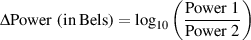 | (2.18) |
Let’s leave the subject for a minute and talk about measurements. Our basic unit of
length is the metre (m). If I were to talk about the distance between the wall and me, I
would measure that distance in metres. If I were to talk about the distance between
Newfoundland and me, I would not use metres, I would use kilometres. Why? Because if
I were to measure the distance between Newfoundland and my house in Denmark in
metres the number would be something like 4,176,120 m. This number is too big, so I
say I’ll measure it in kilometres. I know that 1 km = 1000 m therefore the distance
between Newfoundland and me is 4,176,120 m / 1 000 m/km = 4,176 km. The same
would apply if I were measuring the length of a pencil. I would not use metres because
the number would be something like 0.15 m. It’s easier to think in centimetres or
millimetres for small distances – all we’re really doing is making the number look
nicer.
The same applies to Bels. It turns out that if we use the above equation, we’ll start
getting small numbers. Too small for comfort; so instead of using Bels, we use decibels
or dB. Now all we have to do is convert.
There are 10 dB in a Bel, so if we know the number of Bels, the number of decibels
is just 10 times that. So:
 | (2.19) |
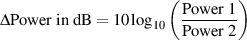 | (2.20) |
So that’s how you calculate dB when you have two different amounts of power and
you want to find the difference between them. The point that I’m trying to overemphasize
thus far is that we are dealing with power measurements. We know that power is
measured in watts (or Joules per second if you’re reading an older book) so we
use the above equation only when the ratio is comparing two measurements in
watts.
What if we wanted to calculate the difference between two voltages (or electrical
pressures)? Well, Watt’s Law says that:
 | (2.21) |
or
 | (2.22) |
Therefore, if we know our two voltages (V1 and V2) and we know the resistance
stays the same:
That’s it! (Finally!) So, the moral of the story is, if you want to compare
two voltages and express the difference in dB, you have to go through that last
equation.
Remember, voltage is analogous to pressure. So if you want to compare two
pressures (like 20*10-6 Pa and 200000000*10-6 Pa) you have to use the same
equation, just substitute V1 and V2 with P1 and P2 like this:
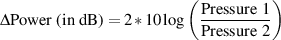 | (2.31) |
This is all well and good if you have two measurements (of power, voltage or
pressure) to compare with each other, but what about all those books that say something
like “a jet at takeoff is 140 dB loud.” What does that mean? Well, what it really means is
“the sound a jet makes when it’s taking off is 140 dB louder than...” Doesn’t make a
great deal of sense... Louder than what? The first measurement was the sound
pressure of the jet taking off, but what was the second measurement with which it’s
compared?
This is where we get into variations on the dB. There are a number of different types
of dB which have references (second measurements) already supplied for you. We’ll do
them one by one.
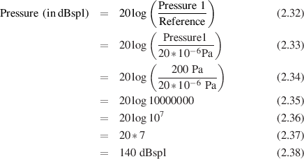
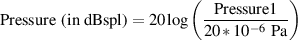
2.2.3 dBspl
The dBspl is a measurement of sound pressure (spl stand for Sound Pressure Level).
What you do is take a measurement of, say, the sound pressure of a jet at takeoff
(measured in Pa). This provides Pressure1. Our reference Pressure2 is given as the sound
pressure of the softest sound you can hear, which we have already said is 20*10-6
Pa.
Let’s say we go to the end of an airport runway with a sound pressure meter and
measure a jet as it flies overhead. Let’s also say that, hypothetically, the sound pressure
turns out to be 200 Pa. Let’s also say we want to calculate this into dBspl. So, the sound
of a jet at takeoff is :
So what we’re saying is that a jet taking off is 140 dBspl which means “the
sound pressure of a jet taking off is 140 dB louder than the softest sound I can
hear.”
2.2.4 dB HL
This issue is covered in Section 5.4.2.
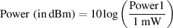
2.2.5 dBm
When you’re measuring sound pressure levels, you use a reference based on the
threshold of hearing (20*10-6 Pa) which is fine, but what if you want to measure the
electrical power output of a piece of audio equipment? What is the reference that you use
to compare your measurement? Well, in 1939, a bunch of people sat down at a
table and decided that when the needles on their equipment read 0 VU, then
the power output of the device in question should be 0.001 W or 1 milliwatt
(mW). Now, remember that the power in watts is dependent on two things – the
voltage and the resistance (Watt’s law again). Back in 1939, the impedance of the
input of every piece of audio gear was 600Ω. If you were Sony in 1939 and you
wanted to build a tape deck or an amplifier or anything else with an input, the
impedance across the input wire and the ground in the connector would have to be
600Ω.
As a result, people today (including me until my error was spotted by Ray Rayburn)
believe that the dBm measurement uses two standard references – 1 mW across a 600Ω
impedance. This is only partially the case. We use the 1 mW, but not the 600Ω. To quote
John Woram, “...the dBm may be correctly used with any convenient resistance or
impedance.” [Woram, 1989]
By the way, the m stands for milliwatt.
Now this is important: since your reference is in mW we’re dealing with power.
Decibels are a measurement of a power difference, therefore you use the following
equation:
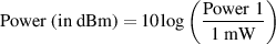 | (2.39) |
Where Power1 is measured in mW.
What’s so important? There’s a 10 in there and not a 20. It would be 20 if we were
measuring pressure, either sound or electrical, but we’re not. We’re measuring
power.
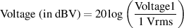
2.2.6 dBV
Nowadays, the 600Ω specification doesn’t apply anymore. The input impedance of a tape
deck you pick up off the shelf tomorrow could be anything – but it’s likely to be pretty
high, somewhere around 10 kΩ. When the impedance is high, the dissipated power is
low, because power is inversely proportional to the resistance. Therefore, there may be
times when your power measurement is quite low, even though your voltage is pretty
high. In this case, it makes more sense to measure the voltage rather than the power. Now
we need a new reference, one in volts rather than watts. Well, there’s actually two
references... The first one is 1 Vrms. When you use this reference, your measurement is
in dBV.
So, you measure the voltage output of your piece of gear – let’s say a mixer, for
example, and compare that measurement with the 1 Vrms reference, using the following
equation.
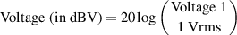 | (2.40) |
Where Voltage1 is measured in Vrms.
Now this time it’s a 20 instead of a 10 because we’re measuring pressure and not
power. Also note that the dBV does not imply a measurement across a specific
impedance.
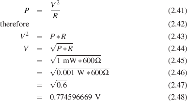
2.2.7 dBu
Let’s think back to the 1mW into 600Ω situation. What will be the voltage required to
generate 1mW in a 600Ω resistor?
Therefore, the voltage required to generate the reference power was about 0.775
Vrms. Nowadays, we don’t use the 600Ω impedance anymore, but the rounded-off value
of 0.775 Vrms was kept as a standard reference. So, if you use 0.775 Vrms as your
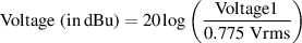
reference voltage in the equation like this:
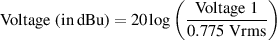 | (2.49) |
your unit of measure is called dBu. Where Voltage1 is measured in Vrms.
(It used to be called dBv, but people kept mixing up dBv with dBV and that
couldn’t continue, so they changed the dBv to dBu instead. You’ll still see dBv
occasionally – it is exactly the same as dBu... just different names for the same
thing.)
Remember – we’re still measuring pressure so it’s a 20 instead of a 10, and, like the
dBV measurement, there is no specified impedance.
2.2.8 dBFS
The dBFS designation is used for digital signals, so we won’t talk about them here.
They’re discussed later in Chapter 10.1.
2.2.9 Addendum: “Professional” vs. “Consumer” Levels
Once upon a time you may have learned that “professional” gear ran at a nominal
operating level of +4 dB compared to “consumer” gear at only -10 dB. (Nowadays, this
seems to be the only distinction between the two...) What few people ever notice is that
this is not a 14 dB difference in level. If you take a piece of consumer gear
outputting what it thinks is 0 dB VU (0 dB on the VU meter), and you plug
it into a piece of pro gear, you’ll find that the level is not -14 dB but -11.79
dB VU... The reason for this is that the professional level is +4 dBu and the
consumer level -10 dBV. Therefore we have two separate reference voltages for each
measurement.
0 dB VU on a piece of pro gear is +4 dBu which in turn translates to an actual
voltage level of 1.228 Vrms. In comparison, 0 dB VU on a piece of consumer gear is -10
dBV, or 0.316 Vrms. If we compare these two voltages in terms of decibels, the result is a
difference of 11.79 dB.
One other thing to remember is that, typically, professional gear uses balanced
signals (this term will be discussed and defined in Section 6.5.2) on XLR connectors
whereas consumer gear uses unbalanced signals on phono (RCA) or 1/4” jacks. If you’re
measuring, then the +4 dBu signal is between the hot and cold pins on the XLR (pins 2
and 3 respectively). If you measure between either of those pins and ground
(pin 1) then you’ll be 6 dB lower. In the case of consumer gear, you measure
between the signal (the pin on a phono connector, the tip on a 1/4” jack) and
ground.
2.2.10 The Summary
dBspl
 | (2.50) |
where Pressure1 is measured in Pa.
dBm
 | (2.51) |
where Power1 is measured in mW.
dBV
 | (2.52) |
where Voltage1 is measured in Vrms.
dBu
 | (2.53) |
where Voltage1 is measured in Vrms.
2.3 Basic Circuits / Series vs. Parallel
2.3.1 Introduction
Picture it – you’re getting a shower one morning and someone in the bathroom
downstairs flushes the toilet... what happens? You scream in pain because you’re
suddenly deprived of cold water in your comfortable hot / cold mix... Not good. Why
does this happen? It’s simple... It’s because you were forced to share cold water without
being asked for permission. Essentially, we can pretend (for the purposes of this
example...) that there is a steady pressure pushing the flow of water into your
house. When the shower and the toilet are asking for water from the same source
(the intake to your house) then the water that was normally flowing through
only one source suddenly goes in two directions. The flow is split between two
paths.
How much water is going to flow down each path? That depends on the amount of
resistance the water “sees” going down each path. The toilet is probably going to have a
lower “resistance” to impede the flow of water than your shower head, and so more water
flows through the toilet than the shower. If the resistance of the shower was
smaller than the toilet, then you would only be mildly uncomfortable instead of
jumping through the shower curtain to get away from the boiling water... In
addition, the toilet would take longer to fill than it usually does when no one is
showering.
2.3.2 Series circuits – from the point of view of the current
Think back to the tanks connected by a pipe with a restriction in it described in Chapter
2.1. All of the water flowing from one tank to the other must flow through the pipe, and
therefore, through the restriction. The flow of the water is, in fact, determined by the
resistance of the restriction (we’re assuming that the pipe does not impede the flow of
water... just the restriction...)
What would happen if we put a second restriction on the same pipe? The water
flowing through the pipe from tank to tank now “sees” a single, bigger resistance, and
therefore flows more slowly through the entire pipe.
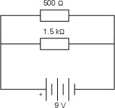
The same is true of an electrical circuit. If we connect two resistors, end to end, and
connect them to a battery as is shown in the diagram below, the current must flow from
the positive battery terminal through the fist resistor, through the second resistor, and into
the negative terminal of the battery. Therefore the current leaving the positive
terminal “sees” one big resistance equivalent to the added resistances of the two
resistors.
What we are looking at here is called an example of resistors connected in series.
What this essentially means is that there are a series of resistors that the current must
flow through in order to make its way through the entire circuit.
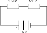
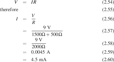
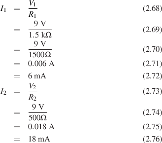
So, how much current will flow through this system? That depends on the two
resistances. If we have a 9 V battery, a 1.5 kohm resistor and a 500 Ω resistor, then the
total resistance is 2 kohms. From there we can just use Ohm’s law to figure out the total
current running through the system.
Remember that this is not only the current flowing through the entire system, it’s also
therefore the current running through each of the two resistors. This piece of
information allows us to go on to calculate the amount of voltage drop across each
resistor.
2.3.3 Series circuits – from the point of view of the voltage
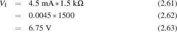
Since we know the amount of current flowing though each of the two resistors, we can
use Ohm’s law to calculate the voltage drop across each of them. Going back to our
original example used above, and if we label our resistors. (R1 = 1.5 kΩ and
R2 = 500Ω)
V1 = I1R1 (This means the voltage drop across R1 = the current through R1 times the
resistance of R1)
Therefore the voltage drop across R1 is 6.75 V.
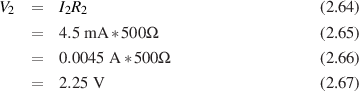
Now we can do the same thing for R2 ( remember, it’s the same current...)
So the voltage drop across R2 is 2.25 V. An interesting thing to note here is that the
voltage drop across R1 and the voltage drop across R2, when added together, equal 9 V. In
fact, in this particular case, we could have simply calculated one of the two voltage drops
and then simply subtracted it from the voltage produced by the battery to find the second
voltage drop.
2.3.4 Parallel circuits – from the point of view of the voltage
Now let’s connect the same two resistors to the battery slightly differently. We’ll put
them side by side, parallel to each other, as shown in the diagram below. This
configuration is called parallel resistors and their effect on the current and voltage in the
circuit is somewhat different than when they were in series...
Look at the connections between the resistors and the battery. They are directly
connected, therefore we know that the battery is ensuring that there is a 9 V voltage drop
across each of the resistors. This is a state imposed by the battery, and you simply
expected to accept it as a given... (just kidding...)
The voltage difference across the battery terminals is 9 V – this is a given
fact which doesn’t change whether they are connected with a resistor or not.
If we connect two parallel resistors across the terminals, they still stay 9 V
apart.
If this is causing some difficulty, think back to the example at the top of this page
where we had a shower running while a toilet was flushing in the same house. The water
pressure supplied to the house didn’t change... It’s the same thing with a battery and two
parallel resistors.
2.3.5 Parallel circuits – from the point of view of the current
Since we know the amount of voltage applied across each resistor (in this case, they’re
both 9 V) then we can again use Ohm’s law to determine the amount of current flowing
though each of the two resistors.
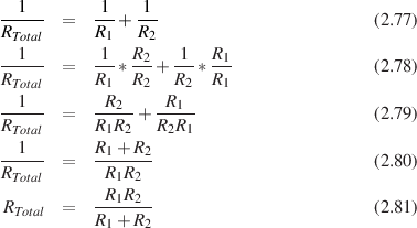
One way to calculate the total current coming out of the battery here is to calculate
the two individual currents going through the resistors, and adding them together.
This will work, and then from there, we can calculate backwards to figure out
what the equivalent resistance of the pair of resistors would be. If we did that
whole procedure, we would find that the reciprocal of the total resistance is
equal to the sum of the reciprocals of the individual resistors. (huh?) It’s like
this...
2.3.6 Suggested Reading List
2.4 Capacitors
Let’s go back a couple of chapters to the concept of a water pump sending water out its
output through a pipe which has a constriction in it back to the input of the pump. We
equated this system with a battery pushing current through a wire and resistor. Now,
we’re replacing the restriction in the water pipe with a couple of waterbeds. Stay with me
here – this will make sense, I promise.
If the input of the water pump is connected to one of the waterbeds and the output of
the pump is connected to the other waterbed, and the output waterbed is placed on top of
the input waterbed, what will happen? Well, if we assume that the two waterbeds have
the same amount of water in them before we turn on the pump (therefore the water
pressure in the two are the same... sort of...) , then, after the pump is turned on, the
water is drained from the bottom waterbed and placed in the top waterbed.
This means that we have a change in the pressure difference between the two
beds (The upper waterbed having the higher pressure). This difference will
increase until we run out of water for the pump to move. The work the pump is
doing is assisted by the fact that, as the top waterbed gets heavier, the water
is pushed out of the bottom waterbed. Now, what does this have to do with
electricity?
We’re going to take the original circuit with the resistor and the battery and we’re
going to add a device called a capacitor in series with the resistor. A capacitor is a
device with two metal plates that are placed very close together, but without
touching. There’s a wire coming off of each of the two plates. Each of these
plates, then can act as a reservoir for electrons – we can push extra ones into a
plate, making it negative (by connecting the negative terminal of a battery to
it), or we can take electrons out, making the plate positive (by connecting the
positive terminal of the battery to it). Remember though that electrons, and the
lack-of-electrons (holes) are mutually attracted to each other. As a result, the extra
electrons in the negative plate are attracted to the holes in the positive plate. This
means that the electrons and holes line up on the sides of the plates closest to the
opposite plate – trying desperately to get across the gap. The narrower the gap,
the more attraction, therefore the more electrons and holes we can pack in the
plates. Also, the bigger the plates, the more electrons and holes we can get in
there.
This device has the capacity to store quantities of electrons and holes – that’s why we
call them capacitors. The value of the capacitor, measured in Farads (abbreviated F) is a
measure of its capacity to hold electrons (we’ll leave it at that for now). That capacitance
is determined by two things essentially – both physical attributes of the device. The first
is the size of the plates – the bigger the plates, the bigger the capacitance. For big caps,
we take a couple of sheets of metal foil with a piece of non-conductive material
sandwiched between them (called the dielectric) and roll the whole thing up like a
sleeping bag being stored for a hike – put the whole thing in a little can and let the
wires stick out of the ends (or one end). The second attribute controlling the
capacitance is the gap between the plates (the smaller the gap, the bigger the
capacitance).
The reason we use these capacitors is because of a little property that they have
which could almost be considered a problem – you can’t dump all the electrons you want
to through the wire into the plate instantaneously. It takes a little bit of time, especially if
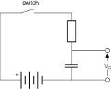
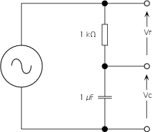
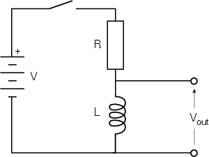
we restrict the current flow a bit with a resistor. Let’s take a circuit as an example. We’ll
connect a switch, a resistor, and a capacitor all in series with a battery, as is shown in
Figure 2.12.
Just before we close the switch, let’s assume that the two plates of the capacitor have
the same number of electrons and holes in them – therefore they are at the same potential
– so the voltage across the capacitor is 0 V (In other words, they have the same electrical
pressure.). When we close the switch, the electrons in the negative terminal want to flow
to the top plate of the cap to meet the holes flowing into the bottom plate. Therefore,
when we first close the switch, we get a surge of current through the circuit which
gradually decreases as the voltage across the capacitor is increased. The more the
capacitor fills with holes and electrons. the higher the voltage across it, and
therefore the smaller the voltage across the resistor – this in turn means a smaller
current.
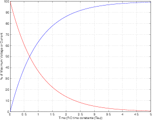
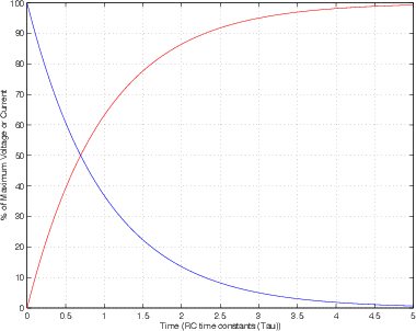
If we were to graph this change in the flow of current over time, it would look like
the red line in Figure 2.13:
As you can see, the longer in time after the switch has been closed, the smaller the
current. The graph of the change in voltage over time would be exactly opposite to this,
plotted as the blue line in Figure 2.13.
In case you want to be a geek and calculate these values, you can use the following
equations – I’m just putting these two in for reference purposes, not because you need to
know or understand them:
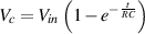 | (2.82) |
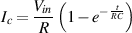 | (2.83) |
Where Vc is the instantaneous voltage across the capacitor, Vin is the instantaneous
voltage applied to the whole circuit, e is approximately 2.718, R is the resistance
of the resistor in Ω, C is the capacitance of the capacitor in Farads, Ic is the
instantaneous current flowing through the resistor and into the capacitor and t is time in
seconds.
You may notice that in most books, the time axis of the graph is not marked in
seconds but in something that looks like a τ – it’s called tau (that’s a Greek letter and not
a Chinese word, in case you’re thinking that I’m going to make a joke about Winnie the
Pooh... It’s also pronounced differently – say “tao” not “dao”). Tau is the symbol for
something called a time constant, which is determined by the value of the capacitor and
the resistor, as in Equation 2.84:
 | (2.84) |
As you can see, if either the resistance or the capacitance is increased, the RC time
constant goes up. “But what’s a time constant?” I hear you cry... Well, a time constant is
the time it takes for the voltage to reach 63.2% of the voltage applied to the capacitor.
After 2 time constants, we’ve gone up 63.2% and then 63.2% of the remaining
36.8%, which means we’re at 86.5%... Once we get to 5 time constants, we’re
at 99.3% of the voltage and we can consider ourselves to have reached our
destination. (In fact, we never really get there – we just keep approaching the voltage
forever.)
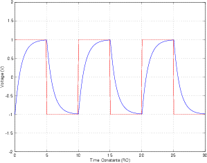
So, this is all very well if our voltage source is providing us with a suddenly applied
DC, but what would happen if we replaced our battery with a square wave and monitored
the voltage across and the current flowing into the capacitor? Well, the output would look
something like Figure 2.14 (assuming that the period of the square wave = 10 time
constants).
What’s going on? Well, the voltage is applied to the capacitor, and it starts charging,
initially demanding lots of current through the resistor, but asking for less and less all the
time. When the voltage drops to the lower half of the square wave, the capacitor starts
charging (or discharging) to the new value, initally demanding lots of current in the
opposite direction and slowly reaching the voltage. Since I said that the period of the
square wave is 10 time constants, the voltage of the capacitor just reaches the voltage of
the function generator (5 time constants...) when the square wave goes to the other
value.
Consider that, since the circuit is rounding off the square edges of the initially
applied square wave, it must be doing something to the frequency response – but we’ll
worry about that later.
Let’s now apply an AC sine wave to the input of the same circuit and look at what’s
going on at the output. The voltage of the function generator is always changing, and
therefore the capacitor is always being asked to change the voltage across it. However, it
is not changing nearly as quickly as it was with the square wave. If the change in voltage
over time is quite slow (therefore, a low frequency sine wave) the current required
to bring the capacitor to its new (but always changing) voltage will be small.
The higher the frequency of the sine wave at the input, the more quickly the
capacitor must change to the new voltage, therefore the more current it demands.
Therefore, the current flowing through the circuit is dependent on the frequency – the
higher the frequency, the higher the current. If we think of this another way,
we could pretend that the capacitor is a resistor which changes in value as the
frequency changes – the lower the frequency, the bigger the resistor, because the
smaller the current. This isn’t really what’s going on, but we’ll work that out in a
minute.
The lower the frequency, the lower the current – the smaller the capacitor the lower
the current (because it needs less current to change to the new voltage than
a bigger capacitor). Therefore, we have a new equation which describes this
relationship:
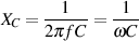 | (2.85) |
Where f is the frequency in Hz, C is the capacitance in Farads, and π is
3.14159264...
What’s XC? It’s something called the capacitive reactance of the capacitor, and it’s
expressed in Ω. It’s not the same as resistance for two reasons – firstly, resistance
burns power (lost as heat) if it’s resisting the flow of current; when current is
impeded by capacitic reactance, there is no power lost. It’s also different from a
resistor becasue there is a different relationship between the voltage and the
current flowing through (or into) the device. For resistors, Ohm’s Law tells
us that V=IR, therefore if the resistor stays the same and the voltage goes up,
the current goes up at the same time. Therefore, we can say that, when an AC
voltage is applied to a resistor, the flow of current through the resistor is in
phase with the voltage. (when V is 0, I is 0, when V is maximum, I is maximum
and so on). In a capacitive circuit (one where the reactance of the capacitor is
much greater than the resistance of the resistor and the two are in ...) the current
preceeds the voltage (remember the time constant curves – voltage changes
slowly, current changes quickly...) by 90∘. This also means that the voltage
across the resistor is 90∘ ahead of the voltage across the capacitor (because the
voltage across the resistor is in phase with the current through it and into the
capacitor).
If this is a little tough to follow, try thinking of it a different way... Stand in a
swimming pool up to your neck in water and take a dinner plate and hold it in your hands
like you would hold the steering wheel of a car. Now start pushing and pulling the plate
forwards and backwards – you’ll notice that this is hard to do because the water in
the pool resists the movement of the plate. Now think about the relationship
between where the plate is (its displacement), its speed and direction of travel (its
velocity), and whether you’re pushing or pulling (your force). These three things
are illustrated (but not to scale) in Figure 2.15. Notice that while the plate is
moving away from you, you’re pushing. This is true whether the plate is near
to you or far from you – your force is dependent on the velocity of the plate.
One other thing to ask is where all your hard work is going – it’s being used
to push water out of the way. In other words, you’re doing a lot of work for
nothing.
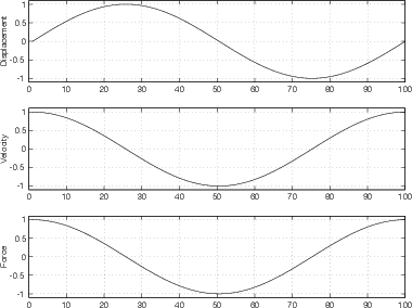
Now get out of the pool and stand in front of a concrete wall with a spring sticking
straight out of it. Glue the bottom of your dinner plate to the spring so that if you push
the plate, it moves towards the wall and squeezes the spring. If you pull the plate, it
moves towards you away from the wall, and expands the spring. Now think about the
relationship between the plate’s displacement and velocity and your force once more.
This is illustrated in Figure 2.16. You’ll notice that it’s a little different than when you
were in the swimming pool. Now, your force is dependent on the displacement of the
plate (since you’re doing all the work to overcome the force of the spring). If the plate
has moved away from you, you’re pushing to overcome the compression of the spring –
this is true regardless of whether the plate is moving away from or towards
you. In addition, the force that you’re putting on the plate is not lost. You’re
storing energy in the spring instead of just losing it as you were in the swimming
pool
Let’s get back to the circuit we were talking about before all of this dinner plate
stuff... As far as the function generator is concerned, it doesn’t know whether
the current it’s being asked to supply is determined by resistance or reactance
– all it sees is some THING out there, impeding the current flow differently
at different frequencies (the lower the frequency, the higher the impedance).
This impedance is not simply the addition of the resistance and the reactance,
because the two are not in phase with each other – in fact they’re 90∘ out of
phase. The way we calculate the total impedance of the circuit is by finding the
square root of the sum of the squares of the resistance and the reactance or
:
 | (2.86) |
Where Z is the impedance of the RC combination, R is the resistance of the resistor,
and XC is the capacitive reactance, all expressed in Ω.
Remember back to Pythagoras – that same equation above is the one we use to find
the length of the hypotenuse of a right triangle (a triangle whose legs are 90∘
apart) when we know the lengths of the legs. Get it? Voltages are 90∘ apart,
legs are 90∘ apart. If you don’t get it, not to worry, it’s explained in Section
2.5.
Also, remember that, as frequency goes up, the XC goes down, and therefore the Z
goes down. If the frequency is 0 Hz (or DC) then the XC is ∞ Ω, and the circuit is
no longer closed – no current will flow. This will come in handy in the next
chapter.
As for the combination of capacitors in series and parallel, it’s exactly the same
equations as for resistors except that they’re opposite. If you put two capacitors in
parallel – the total capacitance is bigger... in fact it’s the addition of the two capacitances
(because you’re effectively making the plates bigger). Therefore, in order to calculate the
total capacitance for a number of capacitors connected in parallel, you use Equation
2.87.
 | (2.87) |
If the capacitors are in series, then you use the equation
 | (2.88) |
Note that both of these equations are very similar to the ones for resistors, except that
we use them “backwards.” That is to say that the equations for series resistors is the same
as for parallel capacitors, and the one for parallel resistors is the same as for series
capacitors.
2.4.1 Electrolytic Capacitors
There is a specific type of capacitor called an electrolytic capacitor – so called because it
uses an electrolyte (go look it up...) as the material for one of its plates. This increases
the capacitance of the unit (relative to cap’s that are not electrolytic) for its
size, so you get a bigger capacitor in a smaller package. Because they usually
have a large capacitance, they are usually used in low-frequency circuits (like
power supplies, as we’ll see later) or in keeping DC out of circuits (as we’ll see
later).
The only problem with electrolytic capacitors is that they are usually polarised. This
means that they’re only happy when one plate is at a higher voltage than the other.
When this is true, you’ll see a ”+” sign somewhere on the cap near one of its
two terminals itself to indicate that that terminal should be connected to the
higher voltage. (It might be a ”-” sign instead – you figure it out...) Note that if
you do not make sure that this is obeyed, then th capacitor will start to heat up
internally, then its contents will start to boil. Since the cap is sealed, this will cause
a build-up in pressure that will, eventually, be released... usually with some
violence.
2.4.2 Suggested Reading List
[VanBuskirk, 1953]
[Walter G. Jung, 1980a]
[Walter G. Jung, 1980b]
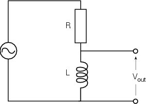
2.5 Passive RC Filters
In the last chapter, we looked at the circuit similar to that in Figure 2.17 and we talked
about the impedance of the RC combination as it related to frequency. Now
we’ll talk about how to harness that incredible power to screw up your audio
signal.
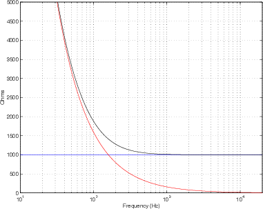
In this circuit, the lower the frequency, the higher the impedance, and therefore the
lower the current flowing through the circuit. If we’re at 0 Hz, there is no current flowing
through the circuit. If we’re at ∞ Hz (this is very high...) then the capacitor has a
capacitive reactance of 0 Ω, and the impedance of the circuit is the resistance of the
resistor. This can be seen in Figure 2.18.
We also talked about how, at low frequencies, the circuit is considered to be
capacitive (because the capacitive reactance is MUCH greater than the resistor value and
therefore the resistor is negligible in comparison.).
When the circuit is capacitive, the current flowing through the resistor into the
capacitor is changing faster than the voltage across the capacitor. We said in
the previous chapter, that, in this case, the current is 90∘ ahead of the voltage.
This also means that the voltage across the resistor (which is in phase with the
current) is 90∘ ahead of the voltage across the capacitor. This is shown in Figure
2.19.
Let’s look at the voltage across the capacitor as we change the voltage. At very low
frequencies, the capacitor has a very high capacitive reactance, therefore the resistance of
the resistor is negligible in comparison. If we consider the circuit to be a voltage divider
(where the voltage is divided between the capacitor and the resistor) then there will
be a much larger voltage drop across the capacitor than the resistor. At DC
(0 Hz) the XC is infinite, and the voltage across the capacitor is equal to the
voltage output from the function generator. Another way to consider this is, if
XC is infinite, then there is no current flowing through the resistor, therefore
there is no voltage drop across is (because 0 V = 0 A * R). If the frequency is
higher, then the reactance is lower, and we have a smaller voltage drop across the
capacitor. The higher we go, the lower the voltage drop until, at ∞ Hz, we have 0
V.
If we were to plot the voltage drop across the capacitor relative to the frequency, it
would, therefore produce a graph like Figure 2.20.
Note that we’re specifying the voltage as a level relative to the input of the circuit,
expressed in dB. The frequency at which the output (the voltage drop across the
capacitor) is 3 dB below the input (that is to say -3 dB) is called the cutoff frequency (fc)
of the circuit. (We may as well start calling it a filter, since it’s filtering different
frequencies differently... since it allows low frequencies to pass through unchanged, we’ll
call it a low-pass filter.)
The fc of the low-pass filter can be calculated if you know the values of the resistor
and the capacitor. The equation is shown in Equation 2.89:
 | (2.89) |
(Note that if we put the values of the resistor and the capacitor from Figure
2.17 – R = 1 kΩ and C = 1 μF ) into this equation, we get 159 Hz. This is the
frequency where R = XC. This is also where the relationship between the input,
and the voltages across the resistor and capacitor behave as is shown in Figure
2.19.)
Where fc is expressed in Hz, R is in Ω and C is in Farads.
At frequencies below  (1 decade below fc – musicians like to think in octaves – 2
times the frequency – engineers like to think in decades, 10 times the frequency) we
consider the output to be equal to the input – therefore at 0 dB. At frequencies 1 decade
above fc and higher, we drop 6 dB in amplitude every time we go up 1 octave, so we say
that we have a slope of -6 dB per octave (this is also expressed as -20 dB per decade – it
means the same thing)
(1 decade below fc – musicians like to think in octaves – 2
times the frequency – engineers like to think in decades, 10 times the frequency) we
consider the output to be equal to the input – therefore at 0 dB. At frequencies 1 decade
above fc and higher, we drop 6 dB in amplitude every time we go up 1 octave, so we say
that we have a slope of -6 dB per octave (this is also expressed as -20 dB per decade – it
means the same thing)
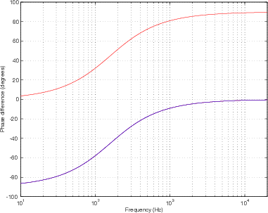
We also have to consider, however, that the change in voltage across the capacitor
isn’t always keeping up with the change in voltage across the function generator. In fact,
at higher frequencies, it lags behind the input voltage by 90∘. Up to 1 decade below fc,
we are in phase with the input, at fc, we are 45∘ behind the input voltage, and at 1 decade
above fc and higher, we are lagging by 90∘. The resulting graph looks like Figure 2.21
:
As is evident in the graph, a lag in the sine wave is expressed as a positive phase,
therefore the voltage across the capacitor goes from 0∘ to 90∘ relative to the input
voltage.
While all that is going on, what’s happening across the resistor? Well, since we’re
considering that this circuit is a fancy type of voltage divider, we can say that if the
voltage across the capacitor is high, the voltage across the resistor is low – if
the voltage across the capacitor is low, then the voltage across the resistor is
high. Another way to consider this is to say that if the frequency is low, then
the current through the circuit is low (because XC is high) and therefore Vr is
low. If the frequency is high, the current is high (because XC is low) and Vr is
high.
The result is Figure 2.20, showing the voltage across the resistor relative to
frequency. Again, we’re plotting the amplitude of the voltage as it relates to the input
voltage, in dB.
Now, of course, we’re looking at a high-pass filter. The fc is again the frequency
where we’re at -3 dB relative to the input, and the equation to calculate it is the same as
for the low-pass filter.
 | (2.90) |
The slope of the filter is now 6 dB per octave (20 dB per decade) because we increase
by 6 dB as we go up one octave... That slope holds true for frequencies up to 1 decade
below fc. At frequencies more than one decade above fc (in mathematical terms, 10 fc),
we are at 0 dB relative to the input.
The phase response is also similar but different. Now the sine wave that we see
across the resistor is ahead of the input. This is because, as we said before, the current
feeding the capacitor preceeds its voltage by 90∘. At extremely low frequencies, we’ve
established that the voltage across the capacitor is in phase with the input – but the
current preceeds that by 90∘. Therefore the voltage across the resistor must preceed the
voltage across the capacitor (and therefore the voltage across the input) by 90∘ (up to
 ).
).
Again, at fc, the voltage across the resistor is 45∘ away from the input, but this time
it is ahead, not behind.
Finally, at fc*10 and above, the voltage across the resistor is in phase with the input.
This all results in the phase response graph shown in Figure 2.21.
As you can see in Figure 2.21, the voltage across the resistor and the voltage across
the capacitor are always 90∘ out of phase with each other, but their relationships with the
input voltage change.
There’s only one thing left that we have to discuss... this is an apparent conflict in
what we have learned (though it isn’t really a conflict...) We know that the fc is the point
where the voltage across the capacitor and the voltage across the resistor are both -3 dB
relative to the input. Therefore the two voltages are equal – yet, when we add
them together, we go up by 3 dB and not 6 dB as we would expect. This is
because the two waves are 90∘ apart – if they were in phase, they would add
to produce a gain of 6 dB. Since they are out of phase by 90∘, their sum is 3
dB.
2.5.1 Another way to consider this...
We know that the voltage across the capacitor and the voltage across the resistor are
always 90∘ apart at all frequencies, regardless of their phase relationships to the input
voltage.
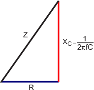
Consider the Resistance and the Capacitive reactance as both providing components
of the impedance, but 90∘ apart. Therefore, we can plot the relationship between these
three using a right triangle as is shown in Figure 2.23.
At this point, it should be easy to see why the impedance is the square root of the
sum of the squares of R and XC. In addition, it becomes intuitive that, as the frequency
goes to ∞ Hz, XC goes to zero and the hypotenuse of the triangle, Z, becomes
the same as R. If the frequency goes to 0 Hz (DC), XC goes to ∞Ω as does
Z.
Go back to the concept of a voltage divider using two resistors. Remember that the
ratio of the two resistances is the same as the ratio of the voltages across the two
resistors.
 | (2.91) |
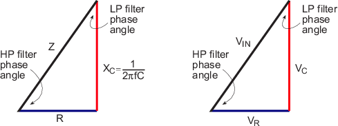
If we consider the RC circuit in Figure 2.17, we can treat the two components in a
similar manner, however the phase change must be taken into consideration. Figure 2.23
shows a triangle exactly the same as that in Figure 2.22 – now showing the
relationship bewteen the input voltage, and the voltages across the resistor and the
capacitor.
So, once again, we can see that, as the frequency goes up, the voltage across
the capacitor goes down until, at ∞ Hz, the voltage across the cap is 0 V and
VIN = VR.
Notice as well that this triangle gives us the phase relationships of the voltages. The
voltage across the resistor and the capacitor are always 90∘ apart, but the phase of these
two voltages in relation to the input voltage changes according to the value of the
capacitive inductance which is, in turn, determined by the capacitance and the
frequency.
So, now we can see that, as the frequency goes down, the current goes down, the
voltage across the resistor goes down, the voltage across the capacitor approaches the
input voltage, the phase of the low-pass filter approaches 0∘ and the phase of the
high-pass filter approaches 90∘. As the frequency goes up, the voltage across the
capacitor goes down, the voltage across the resistor appraoches the input voltage, the
phase of the low-pass filter approaches 90∘ and the phase of the high-pass filter
approaches 0∘.
2.5.2 Suggested Reading List
2.6 Electromagnetism
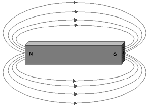
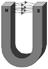
Once upon a time, you did an experiment, probably around grade 3 or so, where you put
a piece of paper on top of a bar magnet and sprinkled iron filings on the paper. The result
was a pretty pattern that spread from pole to pole of the magnet. The iron filings were
aligning themselves along what are called magnetic lines of force. These lines of force
spread out around a magnet and have some effect on the things around them (like iron
filings and compasses for example...) These lines of force have a direction – they go from
the north pole of the magnet to the south pole as shown in Figures 2.24 and
2.25.
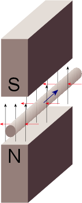
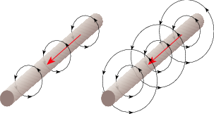
It turns out that there is a relationship between current in a wire and magnetic lines of
force. If we send current through a wire, we generate magentic lines of force that rotate
around the wire. The more current, the more the lines of force expand out from the wire.
The direction of the magnetic lines of force can be calculated using what is probably
the first calculator you ever used... your right hand... Look at Figure 2.26. As
you can see, if your thumb points in the direction of the current and you wrap
your fingers around the wire, the direction your fingers wrap is the direction of
the magnetic field. (You may be asking yourself “so what!?’ – but we’ll get
there...)
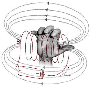
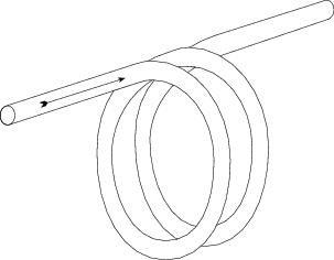
Let’s then, take this wire and make a spring with it so that the wire at one point in
the section of spring that we’ve made is adjacent to another point on the same
wire. The direction of the magnetic field in each section of the wire is then
reinforced by the direction of the adjacent bits of wire and the whole thing
acts as one big magnetic field generator. When this happens, as you can see
below, the coil has a total magnetic field similar to the bar magnet in the diagram
above.
We can use our right hand again to figure out which end of the coil is north and
which is south. If you wrap your fingers around the coil in the direction of the current,
you will find that your thumb is pointing north, as is shown in Figure 2.27. Remember
again, that, if we increase the current through the wire, then the magnetic lines of force
move farther away from the coil.
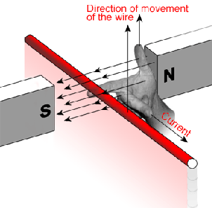
One more interesting relationship between magnetism and current is that if we move
a wire in a magnetic field, the movement will create a current in the wire. Essentially, as
we cut through the magnetic lines of force, we cause the electrons to move in the wire.
The faster we move the wire, the more current we generate. Again, our right hand helps
us determine which way the current is going to flow. If you hold your hand as is shown in
Figure 2.28, point your index finger in the direction of the magnetic lines of
force (N to S...) and your thumb in the direction of the movement of the wire
relative to the lines of force, your middle finger will point in the direction of the
current.
2.6.1 Suggested Reading List
2.7 Inductors
We saw in Section 2.6 that if you have a piece of wire moving through a magnetic field,
you will induce current in the wire. The direction of the current is dependent on the
direction of the magnetic lines of force and the direction of movement of the wire. Figure
2.29 shows an example of this effect.
We also saw that the reverse is true. If you have a piece of wire with current
running through it, then you create a magnetic field around the wire with the
magnetic lines of force going in circles around it. The direction of the magnetic
lines of force is dependent on the direction of the current. The strength of the
magnetic field and, therefore, the distance it extends from the wire is dependent on
the amount of current. An example of this is shown in Figure 2.30 where we
see two different wires with two different magnetic fields due to two different
currents.
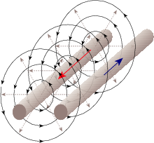
What happens if we combine these two effects? Let’s take a piece of wire and
connect it to a circuit that let’s us have current running through it. Then, we’ll
put a second piece of wire next to the first piece as is shown in Figure 2.31.
Finally, we’ll increase the current over time, so that the magnetic field expands
outwards from the first wire. What will happen? The magnetic lines of force will
expand outwards from around the first wire and cut through the second wire.
This is essentially the same as if we had a constant magnetic field between two
magnets and we moved the wire through it – we’re just moving the magnetic
field instead of the wire. Consequently, we’ll induce a current in the second
wire.
Now let’s go a step further and put a current through the wire on the right that is
always changing – the most common form of this signal in the electrical world
is a sinusoidal waveform that alternates back and forth between positive and
negative current (meaning that it changes direction). Figure 2.32 shows the
result when we put an everyday AC signal into the wire on the left in Figure
2.31.
Let’s take a piece of wire and wind it into a coil consisting of two turns as is shown in
Figure 2.33. One thing to beware of is that we aren’t just wrapping naked wire in a coil -
we have to make sure that adjacent sections of the wire don’t touch each other, so we
insulate the wire using a thin insulation.
Let’s now put that coil in a circuit where it’s in series with a resistor, a voltage supply
and a switch. We’ll also put probes in across the coil to see what the voltage difference
across it is. This circuit will look like Figure 2.34.
Now think about Figure 2.31 as being just the top two adjacent sections of wire in the
coil in Figure 2.33. This should raise a question or two. As we saw in Figure 2.31,
increasing the current in one of the wires results in a current in the other wire in the
opposite direction. If these two wires are actually just two sections of the same coil of
wire, then the current we’re putting through the coil goes through the whole length of
wire. However, if we increase that current, then we induce a current in the opposite
direction on the adjacent wires in the coil, which, as we know, is the same wire.
Therefore, by increasing the current in the wire, we increase the induced current
pushing in the opposite direction, opposing the current that we’re putting in the
wire. This opposing current results in a measurable voltage difference across
the coil that is called back electromotive force or back EMF. This back EMF
is is proportional to the change (and thefore the slope, if we’re looking at a
graph) in the current, not the current itself, since it’s proportional to the speed at
which the wire is cutting through the magnetic field. Therefore, the amount that
the coil (which we’ll now start calling an inductor because we are inducing a
current in the opposite direction), opposes the change in voltage applied to it is
proportional to the frequency, since the higher the frequency, the faster the change in
current.
Armed with this knowledge, let’s think about the circuit in Figure 2.34. Before we
close the switch, there can’t be any current going through the circuit, because it’s not a
circuit... there’s a break in the loop. Then, we close the switch. There is an instantaneous
change in current – or at least there should be, because there is an instantaneous change
in voltage. However, we know that the inductor opposes a change in current – and that
the faster the change, the more it opposes it. Since we closed a switch, we changed the
current infinitely fast (from nothing to something in 0 seconds..) so the inductor opposes
the change with an amount equal to the amount that the current should have
changed. Therefore, nothing happens. For an instant, no current flows through the
system because the inductor becomes a generator pusing current in the opposite
direction.
An instant after this, the voltage has not changed (because the source is DC)
therefore, the attempted current has not changed from the new value, so the inductor
thinks that there has been no change and it opposes the current a little less. As we get
further and further in time from the moment when we close the switch, the inductor
forgets more and more that a change has happened, and pushes current in the opposite
direction less and less, until, finally, it stops pushing back at all (because we have a
constant current, and the magnetic lines of force are not moving any more) and therefore
no back EMF is being generated.
What I just described is plotted as the red line in Figure 2.35
Okay, that looks after the current but what about the voltage difference across the
inductor? Well, we know that if there is no current going through the inductor, then there
is no current going through the resistor. If there is no current going through the resistor,
then there is no voltage difference across it because V = IR. Therefore, when
we first close the switch, all of the voltage of the voltage supply is across the
inductor because there is no difference across the resistor. As we get further and
further in time away from the moment the switch closed, then there is more
and more current going through the resistor, therefore there is more and more
voltage across it, so there is less and less voltage difference across the inductor.
Eventually, the inductor stops pushing back against the flow of current, so the
current just sees the inductor as a piece of wire, therefore, eventually, all of the
voltage drop is across the resistor and there is no voltage difference across the
inductor.
This behaviour is shown as the blue line in Figure 2.35.
You may have already noticed that this graph in Figure 2.35 looks remarkably similar
to the one in Figure 2.13. You’d be right. Notice that the current rises 63.6% in 1 time
period, and that we reach maximum current and 0 voltage difference after 5 time
constants. Notice, however, that a capacitor opposes a change in voltage whereas an
inductor opposes a change in current.
This effect of the inductor opposing a change in current generates something called
inductive reactance, abbreviated XL which is measured in Ω. It’s similar to capacitive
reactance in that it opposes a change in the signal without consuming power. This time,
however, the roles of current and voltage are reversed in that, when we apply a change in
current to the inductor, the current through it changes slowly, but the voltage across it
changes quickly.
The inductance of an inductor is given in henrys, abbreviated H and named after the
American scientist Joseph Henry (1797 - 1878). Generally speaking, the bigger the
inductance in henrys, the bigger the inductor has to be physically. There is one trick that
is used to make the inductor a little more efficient, and that is to wrap the coil around an
iron core. Remember that the wire in the coil is insulated (usually with a kind of varnish
to keep the insulation really thin, and therefore getting the sections of wire as close
together as possible to increase efficiency. Since the wire is insulated, the only thing that
the iron core is doing is to act as a conductor for the magnetic field. This may sound
a little strange at first – so far we have only talked about materials as being
conductors or insulators of electrical current. However, materials can also be
classified as how well they conduct magnetic fields – iron is a very good magnetic
conductor.
Similar to a capacitor, the inductive reactance of an inductor is dependent on the
inductance of the device, in henrys and the frequency of the sinusoidal signal being sent
through it. This is shown in Equation 2.92.
 | (2.92) |
Where L is the inductance of the inductor, in henrys. As can be seen, the inductive
reactance, XL, is proportional to both frequency and inductance (unlike a capacitor, in
which XC is inversely proportional to both frequency and capacitance).
2.7.1 Impedance
Let’s put an inductor in series with a resistor as is shown in Figure 2.36.
Just like the case of a capacitor and a resistor in series (see section 2.4), the resulting
load on the signal generator is an impedance, the result of a combination of a resistance
and an inductance. Similar to what we saw with capacitors, there will be a phase
difference of 90∘ between the voltages across the inductor and the resistor. However,
unlike the capacitor, the voltage across the inductor is 90∘ ahead of the voltage across the
resistor.
Since the resistance and the inductive reactance are 90∘ apart, we can calculate the
total impedance – the load on the signal generator using the Pythagorean Theorem shown
in Equation 2.93 and explained in Section 2.5.
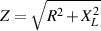 | (2.93) |
2.7.2 RL Filters
We saw in Section 2.5 that we can build a filter using the relationship between the
resistance of a resistor and the capacitive inductance of a capacitor. The same can be
done using a resistor and an inductor, making an RL filter instead of an RC
filter.
Connect an inductor and a resistor in series as is shown in Figure 2.36 and
look at the voltage difference across the inductor as you change the frequency
of the signal generator. If the frequency is very low, then the reactance of the
inductor is practically 0 Ω, so you get almost no voltage difference across it –
therefore no output from the circuit. The higher the frequency, the higher the
reactance. At some frequency, the reactance of the inductor will be the same as the
resistance of the resistor, and the voltages across the two components are the same.
However, since they are 90∘ apart, the voltage across either one will be 0.707 of
the input voltage (or -3 dB). As we go higher in frequency, the reactance goes
higher and higher and we get a higher and higher voltage difference across the
inductor.
This should all sound very familiar. What we have done is to create a first-order
high-pass filter using a resistor and an inductor, therefore it’s called an RL filter. If
we wanted a low-pass filter, then we use the voltage across the resistor as the
output.
The cutoff frequency of an RL filter is calculated using Equation 2.94.
 | (2.94) |
2.7.3 Inductors in Series and Parallel
Finding the total inductance of a number of inductors connected in series or parallel
behave the same way as resistors.
If the inductors are connected in series, then you add the individual inductances as in
Equation 2.95.
 | (2.95) |
If the inductors are connected in parallel, then you use Equation 2.96.
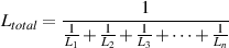 | (2.96) |
2.7.4 Inductors vs. Capacitors
So, if we can build a filter using either an RC circuit or an RL circuit, which should we
use, and why? They give the same frequency and phase responses, so what’s the
difference?
The knee-jerk answer is that we should use an RC circuit instead of an RL
circuit. This is simply because inductors are bigger and heavier than capacitors.
You’ll notice on older equipment that RL circuits were frequently used. This is
because capacitor manufacturing wasn’t great - capacitors would leak electrolytic
over time, thus changing their capacitance and the characteristics of the filter.
An inductor is just a coil, so it doesn’t change over time. However, modern
capacitors are much more stable over long periods of time, so we can trust them in
circuits.
There is a group that claims that they can hear artifacts caused by capacitors in a
circuit. In fact, some companies will even advertise that they have no capacitors in the
signal path as a selling feature.
2.7.5 Suggested Reading List
[Walter G. Jung, 1980a]
[Walter G. Jung, 1980b]
2.8 Transformers
If we take our coil and wrap it around a bar of iron, the iron acts as a conductor for
the magnetic lines of force (not a conductor for the electricity – our wire is
insulated) therefore the lines are concentrated within the bar. (The second right hand
rule still applies for figuring out which way is north – but remember that if
we’re using an AC waveform, the magnetic is changing in strength and polarity
according to the change in the current.) Better yet, we can bend our bar around so it
looks like a donut (mmmmmm donuts...) – that way the lines of force are most
concentrated all the time. If we then wrap another coil around the bar (now
donut-shaped, also known by topologists as toroidal) then the magnetic lines of force
expanding and contracting around the bar will cut through the second coil. This
will generate an alternating current in the second coil, just because it’s sitting
there in a moving magnetic field. The relationship between these two coils is
interesting...
It turns out (we’ll find out in a minute that that was just a pun...) that the power
that we send into the input coil (called the primary coil) of this thing (called a
transformer) is equal to the power that we get out of the second coil (called the
secondary coil). (This is not entirely true – if it were, that would mean that the
transformer is 100% efficient, which is not the case, but we’ll pretend that it
is.)
Also, the ratio of the primary voltage to the secondary voltage is equal to
the ratio of the number of turns of wire in the primary coil to the number of
turns of wire in the secondary coil. This can also be expressed as an equation
:
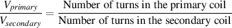 | (2.97) |
Given these two things, we can therefore figure out how much current is flowing into
the transformer based on how much current is demanded of the secondary coil. Looking
at the diagram below :
We know that we have 120 Vrms applied to the primary coil. We therefore know that
the voltage across the secondary coil and therefore across the resistor, is 12 Vrms
because 120 Vrms / 12 Vrms = 10 Turns / 1 Turn.
If we have 12 Vrms across a 15 kohm resistor, then there is 0.8 mA rms flowing
through it (V=IR). Therefore the power consumed by the resistor (therefore the power
output of the secondary coil) is 9.6 mW (P=VI). Therefore the power input of the
transformer is also 9.6 mW. Therefore the current flowing through the primary coil is
0.08 mA rms.
Note that, since the voltage went down by a factor of 10 (the turns ratio of
the transformer) as we went from input to output, the current went up by the
same factor of 10. This is the result of the input power being equal to the output
power.
You can have more than 1 secondary coil on a transformer. In fact, you can have as
many as you want – the power into the primary coil will still be equal to the power of all
of the secondary coils added together. We can also take a tap off the secondary coil at its
half-way point. This is exactly the same as if we had two secondary coils with
exactly the same number of turns, connected to each other in series. In this
case, the centre tap (wire connected to the the half-way point on the coil) is
always half-way in voltage between the two outside legs of the coil. If, therefore,
we use the centre tap as our reference, arbitrarily called 0 V (or ground) then
the two ends of the coil are always an equal voltage “away” from the ground,
but in opposite directions – therefore the two AC waves will be opposite in
polarity.
2.8.1 Suggested Reading List
2.9 Rectifiers and Power Supplies
What use are diodes to us? Well, what happens if we replace the battery from last
chapter’s circuit with an AC source as shown in the Figure 2.38?
Now, when the voltage output of the function generator is positive relative to ground,
it is pushing current through the forward-biased diode and we see current flowing
through the resistor to ground. There’s just the small issue of the 0.6 V drop across
the diode, so until the voltage of the function generator reaches 0.6 V, there
is no current, after that, the voltage drop across the resistor is 0.6 V less than
the function generator’s voltage level until we get back to 0.6 V on the way
down...
When the voltage of the function generator is on the negative half of the wave, the
diode is reverse-biased and no current flows, therefore there is no voltage drop across the
resistor.
This circuit shown in Figure 2.38 is called a half-wave rectifier because it
takes a wave that is alternating between positive and negative voltages and turns
it into a wave that has only positive voltages – but it throws away half of the
wave...
If we instead connect 4 diodes as shown in Figure 2.40, we can use our AC signal
more efficiently.
Now, when the output at the top of the function generator is positive, the current is
pushed through to the diodes and sees two ways to go – one diode (the green
one) will allow current through, while the other (red) one, which is reverse
biased, will not. The current flows through the green diode to a junction where it
chooses between a resistor and another reverse-biased diode (the blue one) ... so it
goes through the resistor (note the direction of the current) and on to another
junction between two diodes. Again, one of these diodes is reverse-biased (red)
so it goes through the other one (yellow) back to the ground of the function
generator.
When the function generator is outputting a negative voltage, the current follows a
different path. The current flows from ground through the blue diode, through the
resistor (note that the direction of the current flow is the same – therefore the
voltage drop is of the same polarity) through the red diode back to the function
generator.
The important thing to notice after all that tracing of signal is that the voltage drop
across the resistor was positive whether the output of the function generator was positive
or negative. Therefore, we are using this circuit to fold the negative half of the original
AC waveform up into the positive side of the fence. This circuit is therefore called a
full-wave rectifier (actually, this particular arrangement of diodes has a specific name
– a bridge rectifier) Remember that at any given time, the current is flowing
through two diodes and the resistor, therefore the voltage drop across the resistor
will be 1.2 V less than the input voltage (0.6 V per diode – we’re assuming
silicon...)
Now, we have this weird bumpy wave – what do we do with it? Easy... if we run it
through a type of low-pass filter to get rid of the spiky bits at the bottom of the
waveform, we can turn this thing into something smoother. We won’t use a
“normal” low-pass filter from Section 2.5, however. We’ll just put a capacitor in
parallel with the resistor. What will this do? Well, when the voltage potential
of the capacitor is less than the output of the bridge rectifier, the current will
flow into the capacitor to charge it up to the same voltage as the output of the
rectifier. This charging current will be quite high, but that’s okay for now... trust
me... When the voltage of the bridge rectifer drops down, the capacitor can’t
discharge back into it, because the diodes are now reverse-biased, so the capacitor
discharges through the resistor according to their time constant (remember?).
Hopefully, before it gets time to discharge, the voltage of the bridge rectifier
comes back up and charges up the capacitor again and the whole cycle repeats
itself.
The end result is that the voltage across the resistor is now a slightly weird AC with a
DC offset, as is shown in Figure 2.44.
The width of the AC of this wave is given as a peak-peak measurement which is a
percentage of the DC content of the wave. The smaller the percentage, the smoother and
therefore better, the waveform.
If we know the value of the capacitor and the resistor, we can calculate the ripple
using the Equation 2.98 :
 | (2.98) |
where f is the frequency of the original waveforem in Hz, R is the value of the
resistor in Ω and C is the value of the capacitor.
All we need to do, therefore, to make the ripple smaller, is to make the capacitor
bigger (the resistor is really not a resistor in a real power supply, its actually something
like a lightbulb or a portable CD player).
Generally, in a real power supply, we’d add one more thing called a voltage regulator
as is shown in Figures 2.45 and 2.46. This is a magic little device which, when fed a
voltage above what you want, will give you what you want, burning off the
excess as heat. They come in two flavours, negative and positive, the positive
ones are designated 78XX where XX is the voltage (for example, a 7812 is
a + 12 V regulator) the negative ones are designated 79XX (ditto... 7918 is
a -18 V regulator.) These chips have 3 pins, one input, one ground and one
output. You feed too much voltage into the input (i.e. 8.5 V into a 7805) and
the chip looks at its ground, gives you exactly the right voltage at the output
and gets toasty. If you use these things (you will) you’ll have to bolt it to a
little radiator or to the chassis of whatever you’re building so that the heat will
dissipate.
A couple of things about regulators : if you reverse-bias them (i.e. try and send
voltage in its output) you’ll break it – probably gonna see a bit of smoke too. Also, they
get cranky if you demand too much current from their output. Be nice. (This is
why you won’t see regulators in a power supply for a power amp which needs
lots-o-current.)
So, now you know how to build a real-live AC to DC power supply just like the pros.
Just use an appropriate transformer instead of a function generator, plug the
thing into the wall (fuses are your friend) and throw away your batteries. The
schematic below is a typical power supply of any device built before switching
power supplies were invented (we’re not going to even try to figure out how they
work).
Below is another variation of the same power supply, but this one uses the centre-tap
as the ground, so we get symmetrical negative and positive DC voltages output from the
regulators.
Suggested Reading List
2.10 Operational Amplifiers
2.10.1 Introduction
If we take enough transistors and build a circuit out of them we can construct a
magic device with three very useful characteristics. In no particular order, these
are
- infinite gain
- infinite input impedance
- zero output impedance
At the outset, these don’t appear to be very useful, however, the device, called an
operational amplifier or op amp, is used in almost every audio component built today. It
has two inputs (one labeled “positive” or “non-inverting” and the other “negative” or
“inverting”) and one output. The op amp measures the difference between the voltages
applied to the two input “legs” (the positive minus the negative), multiples this difference
by a gain of infinity, and generates this voltage level at its output. Of course,
this would mean that, if there was any difference at all between the two input
legs, then the output would swing to either infinity volts (if the level of the
non-inverting input was greater than that of the inverting input) or negative infinity volts
(if the reverse were true). Since we obviously can’t produce a level of either
infinity or negative infinity volts, the op amp tries to do it, but hits a maximum
value determined by the power supply rails that feed it. This could be either a
battery or an AC to DC power supply such as the ones we looked at in Chapter
2.9.
We’re not going to delve into how an op amp works or why – for the purposes of this
book, our time is far better spent simply diving in and looking at how it’s used.
The simplest way to start looking at audio circuits which employ op amps is to
consider a couple of possible configurations, each of which are, in fact, small
circuits in and of themselves that can be combined like Legos to create a larger
circuit.
2.10.2 Schematic representation
We’ll start by looking at how an op amp is represented in a circuit diagram, shown in
Figure 2.47.
Looking at Figure 2.47, the triangle itself is the op amp. It has two signal inputs
(labeled V1 in and V2 in) and one signal output (labeled V out). Notice on the triangle
itself there are small negative and positive signs. These indicate whether the inputs are
inverting or non-inverting. It is standard notation to make the upper input the inverting
input.
There are two additional legs on the op amp, marked +V and -V. These are the
connections for the power supply. Typically in audio applications, these will be
symmetrical – therefore you will have a power supply with + 15 V connected to +V and
-15 V connected to -V (or +/- 18 V or +/- some other voltage).
Notice that there is no connection between the op amp and ground – however, as
we’ll see later, sometimes we may want to connect one of the legs to the ground plane for
one reason or another.
2.10.3 Comparators
The first configuration we’ll look at is a circuit called a comparator. You won’t find this
configuration in many audio circuits (blinking light circuits excepted) but it’s a good way
to start thinking about these devices.
Looking at the above schematic, you’ll see that the inverting input of the op amp is
connected directly to ground, therefore, it remains at a constant 0 V reference level. The
audio signal is fed to the non-inverting input.
The result of this circuit can have three possible states.
- If the audio signal at the non-inverting input is exactly 0 V then it will be
the same as the level of the voltage at the inverting input. The op amp then
subtracts 0 V (at the inverting input, because it’s connected to ground) from
0 V (at the non-inverting input, because we said that the audio signal was at
0 V) and multiplies the difference of 0 V by infinity and arrives at 0 V at the
output. (okay, okay – I know. 0 multipled by infinity is really equal to any
real number, but, in this case, that real number will always be 0)
- If the audio signal is greater than 0 V, then the op amp will subtract 0 V from
a positive number, arriving at a positive value, multiply that result by infinity
and have an output of positive infinity (actually, as high as the op amp can
go, which will really be the voltage of the positive power supply rail)
- If the audio signal is less than 0 V, then the op amp will subtract 0 V from a
negative number, arriving at a negative value, multiply that result by infinity
and have an output of negative infinity (actually, as low as the op amp can
go, which will really be the voltage of the negative power supply rail)
So, if we feed a sine wave with a level of 1 Vp and a frequency of 1 kHz into this
comparator and power it with a 15 V power supply, what we’ll see at the output is a 1
kHz square wave with a level of 15 Vp.
Unless you re a big fan of square waves or very ugly distortion pedals, this circuit
will not be terribly useful to your audio circuits with one noteable exception with we’ll
discuss later. So, how do we use op amps to our advantage? Well, the problem is that the
infinite gain has to be tamed – and luckily this can be done with the helps of just a few
resistors.
2.10.4 Inverting Amplifier
Take a look at the circuit in Figure 2.50.
What do we have here? The non-inverting input of the op amp is permanently
connected to ground, therefore it remains at a constant level of 0 V. The non-inverting
input, on the other hand, is connected to a couple of resistors in a configuration
that sort of resembles a voltage divider. The audio signal feeds into the input
resistor labeled R1. Since the input impedance of the op amp is infinite, all of the
current travelling through R1 caused by the input must be directed through the
second resistor labeled Rf and therefore to the output. The big “problem” here is
that the output of the op amp is connected to its own input and anyone who
works in audio knows that this means one thing... the dreaded monster known
as feedback (which explains the “f” in “Rf” – it’s sometimes known as the
feedback resistor). Well, it turns out that, in this particular case, feedback is
your friend – this is because it is a special brand of feedback known as negative
feedback.
There are a number of ways to conceptualize what s happening in this circuit. Let’s
apply a +1 V DC signal to the input R1 which we’ll assume to be 1 k – what will
happen?
Let’s assume for a moment that the voltage at the inverting input of the op amp is 0 V.
Using Ohm’s Law, we know that there is 1 mA of current flowing through R1. Since
the input impedance of the op amp is infinity, there will be no current flowing
into the amplifier – therefore all of the current must flow through Rf (which
we’ll also make 1 kΩ) as well. Again using Ohm’s Law, we know that there
s 1 mA flowing through a 1 kΩ resistor, therefore there is a 1 V drop across
it. This then means that the voltage at the output of Rf (and therefore the op
amp) is -1 V. Of course, this magic wouldn’t happen without the op amp doing
something...
Another way of looking at this is to say that the op amp “sees” 1 V coming in its
inverting input – therefore it swings its output to negative infinity. That negative infinity
volt output, however, comes back into the inverting input through Rf which causes
the output to swing to positive infinity which comes back into the inverting
input through Rf which causes the output to swing to negative infinity and so on
and so on... All of this swinging back and forth between positive and negative
infinity looks after itself, causing the 1 V input to make it through, inverted to -1
V.
One little thing that’s useful to know – remember that assumption that the level of the
inverting input stays at 0 V? It’s actually a good assumption. In fact, if the voltage level
of the inverting input was anything other than 0 V, the output would swing to one of the
voltage rails. We can consider the inverting input to be at a virtual ground –
“ground” because it stays at 0 V but “virtual” because it isn’t actually connected to
ground.
What happens when we change the value of the two resistors? We change the
gain of the circuit. In the above example, with both R1 and Rf were 1 kΩ and
this resulted in a gain of -1. In order to achieve different gains we follow the
equation:
 | (2.99) |
2.10.5 Non-Inverting Amplifier
There are a couple of advantages of using the inverting amplifier – you can have any gain
you want (as long as it’s negative or zero) and it only requires two resistors. The
disadvantage is that it inverts the polarity of the signal – so in order to maintain the
correct polarity of a device, you need an even number of inverting amplifier circuits, thus
increasing the noise generated by extra components.
It is possible to use a single op amp in a non-inverting configuration as shown in the
schematic in Figure 2.51.
Notice that this circuit is similar to the inverting op amp configuration in that there is
a feedback resistor, however, in this case, the input to R1 is connected to ground and the
signal is fed to the non-inverting input of the op amp.
We know that the voltage at the non-inverting input of the op amp is the same as the
voltage of the signal, for now, let’s say +1 V again. Following an assumption that we
made in the case of the inverting amplifier configuration, we can say that the level of the
two input legs of the op amp are always matched. If this is the case, then let’s follow the
current through R1 and Rf. The voltage across R1 is equal to the voltage of the signal,
therefore there is 1 mA of current flowing though R1, but this time from right to left.
Since the impedance of the input of the op amp is infinite, all of the current flowing
through R1 must be the same as is flowing through Rf. If there is 1 mA of current flowing
through Rf, then there is a 1 V difference across it. Since the voltage at the input
leg side of the op amp is + 1 V, and there is another 1 V across Rf, then the
voltage at the output of the op amp is +2 V, therefore the circuit has a gain of
2.
The result of this circuit is a device which can amplify signals without inverting the
polarity of the original input voltage. The only drawback of this circuit lies in the
fact that the voltages at the input legs of the op amp must be the same. If the
value of the feedback resistor is 0Ω, in other words, a piece of wire, then the
output will equal the input voltage, therefore the gain of the circuit will be 1.
If the value of the feedback resistor is greater than 0Ω, then the gain of the
circuit will be greater than 1. Therefore the minimum gain of this circuit is
1 – so we cannot attenuate the signal as we can with the inverting amplifier
configuration.
Following the above schematic, the equation for determining the gain of the circuit
is
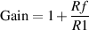 | (2.100) |
2.10.6 Voltage Follower
There is a special case of the non-inverting amplifier configuration which is used
frequently in audio circuitry to isolate signals within devices. In this case, the feedback
“resistor” has a value of 0 Ω – a wire. We also omit the connection between the inverting
input leg and the ground plane. This resistor is effectively unnecessary since
setting the value of Rf to 0 Ω makes the gain equation go immediately to 1.
Changing the value of R1 will have no effect on the gain, whether it’s infinite or
finite, as long as it’s not 0 Ω . Omitting the R1 resistor makes the gain value
infinity.
This circuit will have an output which is identical to the intput voltage,
therefore it is called a voltage follower (also known as a buffer) since it follows the
signal level. The question then is, “what use is it?” Well, it’s very useful if you
want to isolate a signal so that whatever you connect the output of the circuit to
has no effect on the circuit itself. We’ll go into this a little farther in a later
chapter.
2.10.7 Leftovers
There is one of the three characteristics of op amps that we mentioned up front that we
haven’t talked about since. This is the output impedance, which was stated to be 0 Ω .
Why is this important? The answer to this lies in two places. The first is the simple
voltage divider, the second is a block diagram of an op amp. If you look at the diagram in
Figure 2.53, you’ll see that the op amp contains what can be considered as a function
generator which outputs through an internal resistor (the output impedance) to the world.
If we add an external load to the output of the op amp then we create a voltage divider.
If the internal impedance of the op amp is anything other than 0Ω, then the
output voltage of the amplifier will drop whenever a load is applied to it. For
example, if the output impedance of the op amp was 100Ω, and we attached a
100Ω resistor to its output, then the voltage level of the output would be cut in
half.
2.10.8 Mixing Amplifier
How to build a mixer: take an inverting amplifier circuit and add a second input (through
a second resistor, of course...). In fact, you could add as many extra inputs (each with its
own resistor) as you wanted to do. The current flowing through each individual
resistor to the virtual ground winds up at the bottleneck and the total current
flows through the feedback resistor. A schematic of this is shown in Figure
2.54.
The total voltage at the output of the circuit will be:
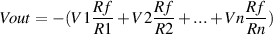 | (2.101) |
As you can see, each input voltage is inverted in polarity (the negative sign at the
beginning of the right side of the equation looks after that) and individually
multiplied by its gain determined by the relationship between its input resistor
and the feedback resistor. This, of course, is a very simple mixing circuit (an
SSL console it isn’t...) but it will work quite effectively with a minimum of
parts.
2.10.9 Differential Amplifier
The mixing circuit in Figure 2.54 adds a number of different signals and outputs the
result (albeit inverted in polarity and possibly with a little gain added for flavour...). It
may also be useful (for a number of reasons that we’ll talk about later) to subtract
signals instead. This, of course, could be done by inverting a signal before adding
them (adding a negative is the same as subtracting...) but you could be a little
more efficient by using the fact that an op amp is a differential amplifier all by
itself.
You will notice in Figure 2.55 that there are two inputs to a single op amp. The result
of the circuit is the difference between the two inputs as can be seen in Equation 2.102.
Usually the gain of the two inputs of the amplifier are set to be equal because the
usual use of this circuit is for balanced inputs which we’ll discuss in a later
chapter.
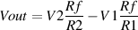 | (2.102) |
2.10.10 Suggested Reading List
2.11 Op Amp Characteristics and Specifications
2.11.1 Introduction
If you get the technical information about an op amp (from the manufacturer’s
datasheets or their website) you’ll see a bunch of specifications that tell you
exactly what to expect from that particular device. Following is a list of specs and
explanations for some of the more important characteristics that you should worry
about.
Most of these definitions are simplified paraphrases of a chapter of an excellent book
called the IC Op-Amp Cookbook written by Walter G. Jung. It used to be published by
SAMS, but now it’s published by Prentice Hall (ISBN 0-13-889601-1) You
should own a copy of this book if you’re planning on doing anything with op
amps.
2.11.2 Maximum Supply Voltage
The supply voltage is the maximum voltage which you can apply to the power supply
inputs of the op amp before it fails. Depending on who made the amplifier and which
model it is, this can vary from ±1 V to ±40 V.
2.11.3 Maximum Differential Input Voltage
In theory, there is no connection at all between the two inputs of an operational amplifier.
If the difference in voltage between the two inputs of the op amp is excessive (on the
order of up to ±30 V) then things inside the op amp break down and current starts to
flow between the two inputs. This is bad – and it happens when the difference in the
voltages applied to the two inputs is equal to the maximum differential input
voltage.
2.11.4 Output Short-Circuit Duration
If you make a direct connection between the output of the amplifier and either the ground
or one of the power supply rails, eventually the op amp will fail. The amount of time this
will take is called the output short-circuit duration, and is different depending on where
the connection is made. (whether it’s to ground or one of the power supply
rails)
2.11.5 Input Resistance
If you connect one of the two input legs of the op amp to ground and then measure the
resistance between the other input leg and ground, you’ll find that it’s not infinite as we
said it would be in the previous chapter. In fact, it’ll be somewhere up around 1MΩ give
or take. This value is known as the “input resistance.”
2.11.6 Common Mode Rejection Ratio (CMRR)
In theory, if we send exactly the same signal to both input legs of an op amp and look at
the output, we should see a constant level of 0 V. This is because the op amp is
subtracting the signal from itself and giving you the result (0 V) multiplied by some gain.
In practice, however, you won’t see a constant 0 V at the output – you’ll see an
attenuated version of the signal that you’re sending into the amplifier’s inputs. The ratio
between the level of the input signal and the level of the resulting output is a
measurement of how much the op amp is able to reject a common mode signal (in other
words, a signal which is common to both input legs). This is particularly useful (as
we’ll see later) in rejecting noise and other unwanted signals on a transmission
line.
The higher this number the better the rejection, and you should see values
in the area of about 100 dB. Be careful though – op amps have very different
CMRR’s for different frequencies (lower frequencies reject better) so take a
look at what frequency you’re talking about when you’re looking at CMRR
values.
2.11.7 Input Voltage Range (Operating Common-Mode Range)
This is simply the range of voltage that you can send to the input terminals while
ensuring that the op amp behaves as you expect it to. If you exceed the input voltage
range, the amplifier could do some unexpected things on you.
2.11.8 Output Voltage Swing
The output voltage swing is the maximum peak voltage that the output can produce
before it starts clipping. This voltage is dependent on the voltage supplied to the op amp
– the higher the supply voltage the higher the output voltage swing. A manufacturer’s
datasheet will specify an output voltage swing for a specific supply voltage – usually
±15 V for audio op amps.
2.11.9 Output Resistance
We said in the last chapter that one of the characteristics of op amps is that they have an
output impedance of 0Ω. This wasn’t really true... In fact, the output impedance of an op
amp will vary from less than 100Ω to about 10kΩ. Usually, an op amp intended for
audio purposes will have an output impedance in the lower end of this scale –
usually about 50Ω to 100Ω or so. This measurement is taken without using a
feedback loop on the op amp, and with small signal levels above a few hundred
Hz.
2.11.10 Open Loop Voltage Gain
Usually, we use op amps with a feedback loop. This is in order to control what we said in
the last chapter was the op amp’s infinite gain. In fact, an op amps does not have an
infinite gain – but it’s pretty high. The gain of the op amp when no feedback look is
connected is somewhere up around 100 dB. Of course, this is also dependent on the load
that the output is driving, the smaller the load, the smaller the output and therefore the
smaller the gain of the entire device.
The open loop voltage gain is a meaurement of the gain of the op amp driving a
specified load when there’s no feedback loop in place (hence the “open loop”). 100 dB is
a typical value for this specification. Its value doesn’t change much with changes in
temperature (unlike some other specifications) but it does vary with frequency. As you go
up in frequency, the gain of the op amp decreases.
2.11.11 Gain Bandwidth Product (GBP)
Eventually, if you keep going up in frequency as you’re measuring the open-loop voltage
gain of the op amp, you’ll reach a frequency where the gain of the system is 1. That is to
say that the input is the same level as the output. If we take the gain at that
frequency (1) and multiply it by the frequency (or bandwidth) we’ll get the Gain
Bandwidth Product. This will then tell you an important characteristic of the op amp,
since the gain of the op amp rolls off at a rate of 6 dB/octave. If you take a
given frequency and divide it by the GBP, you’ll find the open-loop gain at that
frequency.
2.11.12 Slew Rate
In theory, an op amp is able to accurately and instantaneously output a signal which is a
copy of the input, with some amount of gain applied. If, however, the resulting output
signal is quite large, and there are very fast, large changes in that value, the op amp
simply won’t be able to deliver on time. For example, if we try to make the
amplifier’s output swing from -10 V to +10 V instantaneously, it can’t do it –
not quite as fast as we’d like, anyway... The maximum rate at which the op
amp is able to change to a different voltage is called the “slew rate” because
it’s the rate at which the amplifier can slew to a different value. It’s usually
expressed in V/μS – the bigger the number, the faster the op amp. The faster the op
amp, the better it is able to accurately reflect transient changes in the audio
signal.
The slew rate of different op amps varies widely. Typically, you’ll want to see about 5
V/μS or more.
2.11.13 Suggested Reading List
2.12 Practical Op Amp Applications
2.12.1 Active Filters
Frequently, it’s preferable to use active filter designs instead of passive ones. This could
be for a number of reasons. You might want to have the option to add gain in your filter.
Or maybe you don’t want to buffer the filter using two op amps (one on either
end) when you could just use one op amp as part of the circuit (as we’ll see
later).
Butterworth filters
So far, we have looked at only two kinds of low pass and high pass filters. These were
simple passive RC or RL filters. The frequency and phase response characteristics of this
filter design are very predictable and should be intuitively understood before going much
further in this chapter.
There are other types of filter designs that have differing characteristics making
them good for differing applications. One of the most popular filter designs,
widely used in loudspeaker crossovers is called a Butterworth filter. The reason a
Butterworth design is preferred in many cases is due to the fact that it has an
extremely flat passband. We’ll also see in the Section 6.10 on loudspeakers
that the phase response of a Butterworth filter makes it really nice for making
crossovers.
Low Pass (First Order)
Let’s build a simple filter. A first-order Butterworth low pass filter has the same
magnitude and phase response characteristics as a passive RC filter with the exception of
the fact that you can have gain in the passband. Take a look at Figure 2.56 and you’ll see
why this is the case. You’ll notice that this circuit is a combination of two things:
The first is a passive low pass filter (using capacitor C and resistor R). The
second is a non-inverting op amp combination using the op amp and the three
resistors.
The characteristics of this filter can be calculated using the following equations.
Alternately, if you know the characteristics of the filter you want, you can design the
filter using the same equations.
 | (2.103) |
 | (2.104) |
Where GF is the passband gain of the filter
fc is the cutoff frequency of the filter
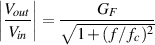 | (2.105) |
 | (2.106) |
Where ϕ is the phase angle
High Pass (First Order)
Equations:
 | (2.107) |
 | (2.108) |
Where GF is the passband gain of the filter
fc is the cutoff frequency of the filter
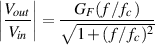 | (2.109) |
How to design a first-order high pass Butterworth filter:
- Determine your cutoff frequency
- Select a mylar or tantalum capacitor with a value of less than about 1 μF.
- Calculate the value of R using R =

- Select values for R1 and R2 (on the order of 10 kΩ or so) to deliver your
desired passband gain.
Low Pass (Second Order)
Equations:
 | (2.110) |
 | (2.111) |
Where GF is the passband gain of the filter
fc is the cutoff frequency of the filter
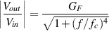 | (2.112) |
Equations:
 | (2.113) |
Note: GF must equal 1.586 in order to have a true Butterworth response[Gayakwad,
1983].
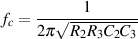 | (2.114) |
Where GF is the passband gain of the filter
fc is the cutoff frequency of the filter
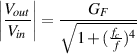 | (2.115) |
How to design a second-order high pass Butterworth filter:
- Determine your cutoff frequency
- Make R2 = R3 = R and C2 = C3 = C
- Select a mylar or tantalum capacitor with a value of less than about 1 μF.
- Calculate the value of R using R =

- Choose a value of R1 that’s less than 100kΩ
- Make Rf = 0.586 R1. Note that this makes your passband gain
approximately equal to 1.586. This is necessary to guarantee a Butterworth
response[Gayakwad, 1983].
2.12.2 Higher-order filters
In order to make higher-order filters, you simply have to connect the filters that you want
in series. For example, if you want a third-order filter, you just take the output of a
first-order filter and feed it into the input of a second-order filter. For a fourth-order filter,
you just cascade two second-order filters and so on. This isn’t exactly as simple as it
seems, however, because you have to pay attention to the relationship of the cutoff
frequencies and passband gains of the various stages in order to make the total filter
behave properly. For more information on this, I’m afraid that you’ll have to look
elsewhere for now... However, if you’re not overly concerned with pinpoint accuracy of
the constructed filter to the theoretical calculated response, you can just use
what you already know and come pretty close to making a workable high-order
filter.
2.12.3 Bandpass filters
Bandpass filters are those that permit a band of frequencies to pass through the filter,
while attenuating signals in frequency bands above and below the passband. These types
of filters should be sub-divided into two categories: those with a wide passband, and
those with a narrow passband.
If the passband of the bandpass filter is wide, then we can create it using a high-pass
filter in series with a low-pass filter. The result will be a signal whose low-frequency
content will be attenuated by the high-pass filter and whose high-frequency content will
be attenuated by the low-pass filter. The result is that the band of frequencies between the
two cutoff frequencies will be permitted to pass relatively unaffected. One of the nice
aspects of this design is that you can have different orders of filters for your high and low
pass (although if they are different, then you have a bit of a weird bandpass
filter...)
If the passband of the bandpass filter is narrow (if the Q is greater than 10), then
you’ll have to build a different circuit that relies on the resonance of the filter in order to
work. Take a look [Gayakwad, 1983] (or any decent book on op amp applications) to see
how this is done.
2.12.4 Suggested Reading List