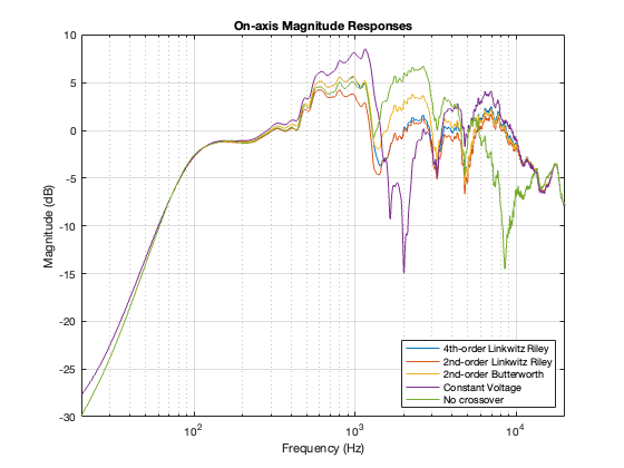
Up to now in this series, we’ve looked at 4 different types of crossover designs:
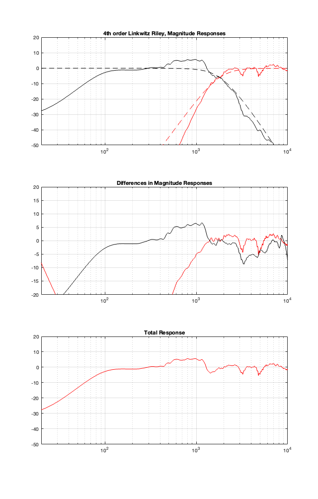
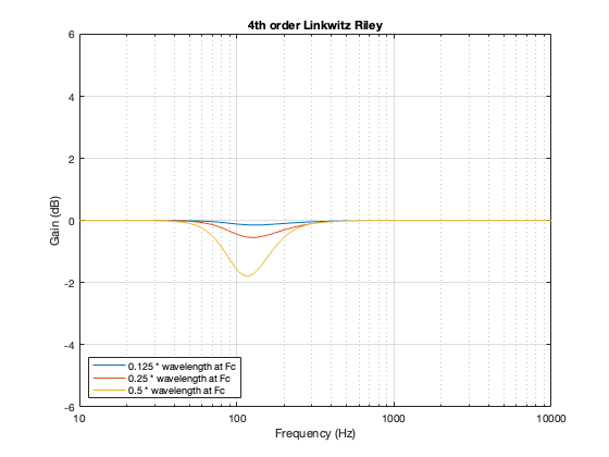
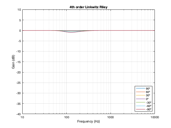
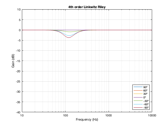
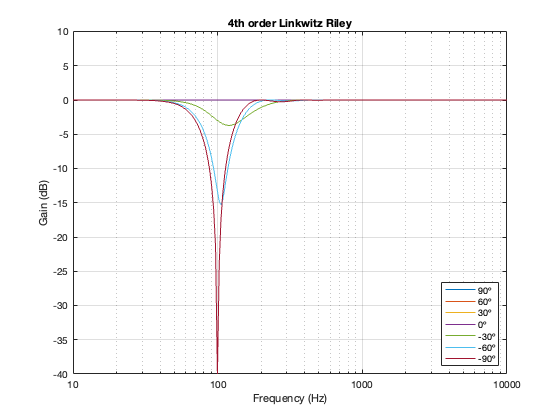
- 4th-order Linkwitz Riley
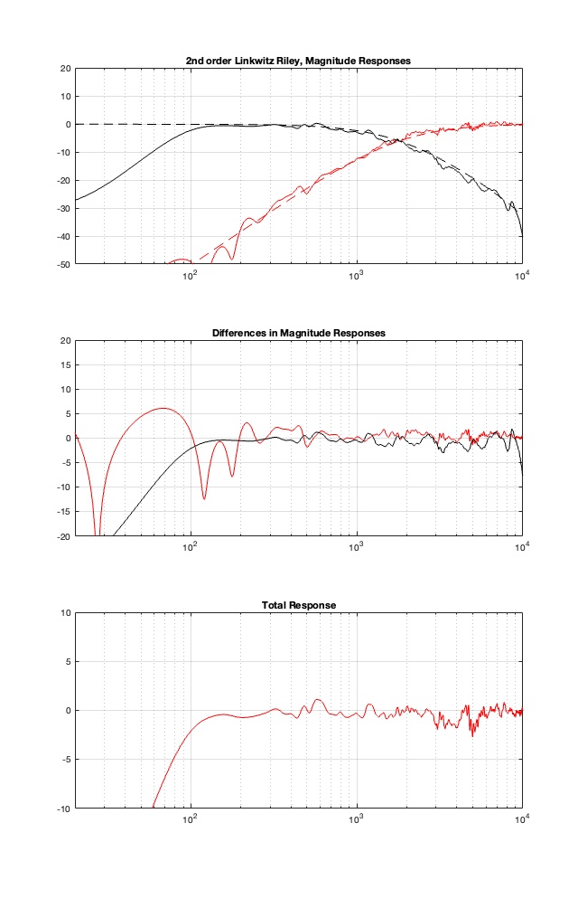
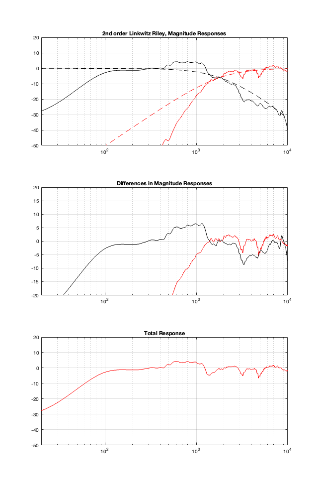
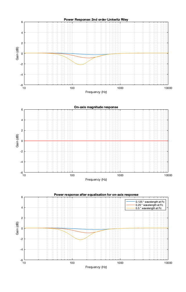
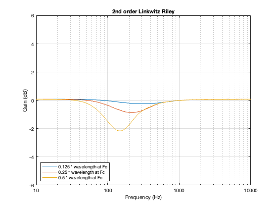
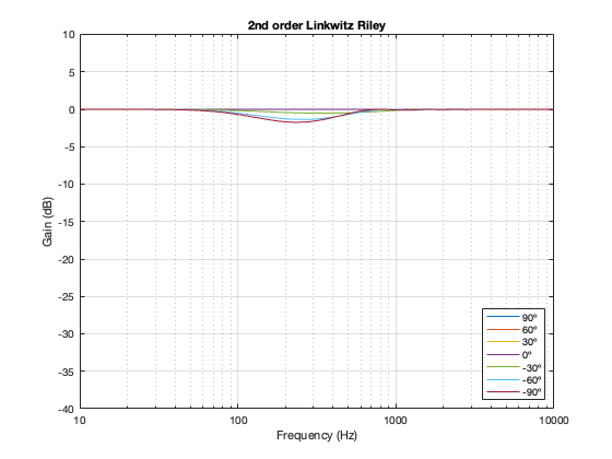
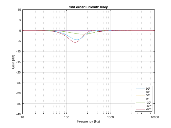
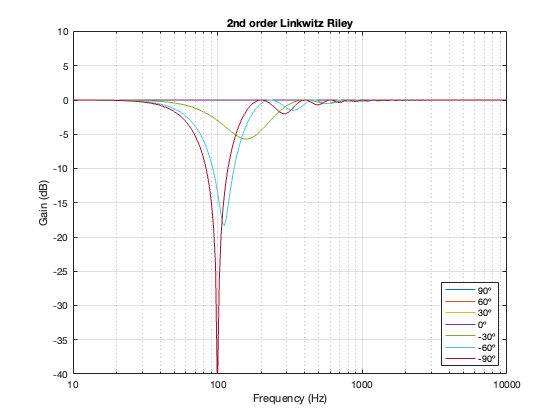
- 2nd-order Linkwitz Riley
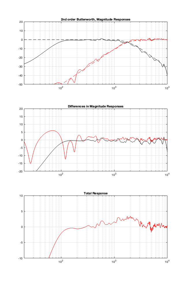
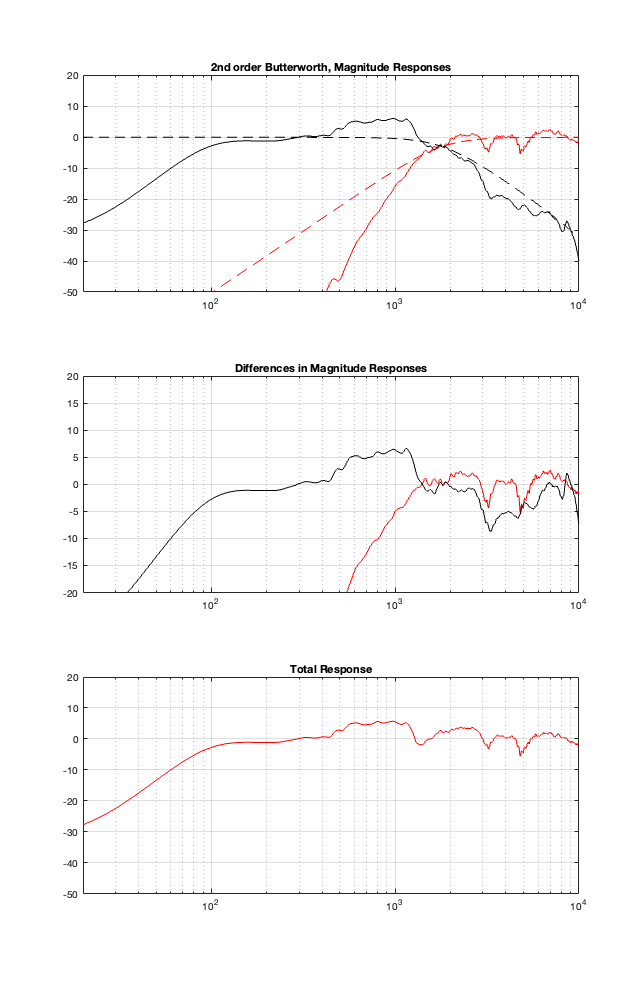
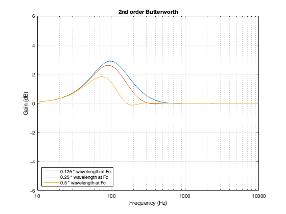
- 2nd-order Butterworth
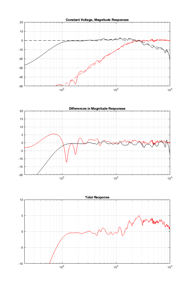
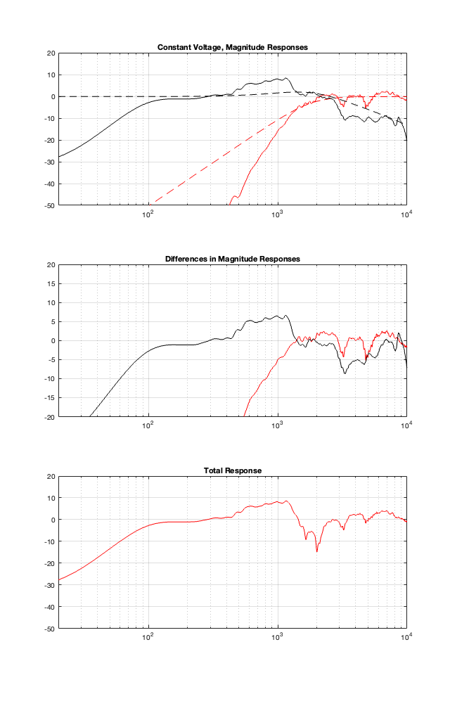
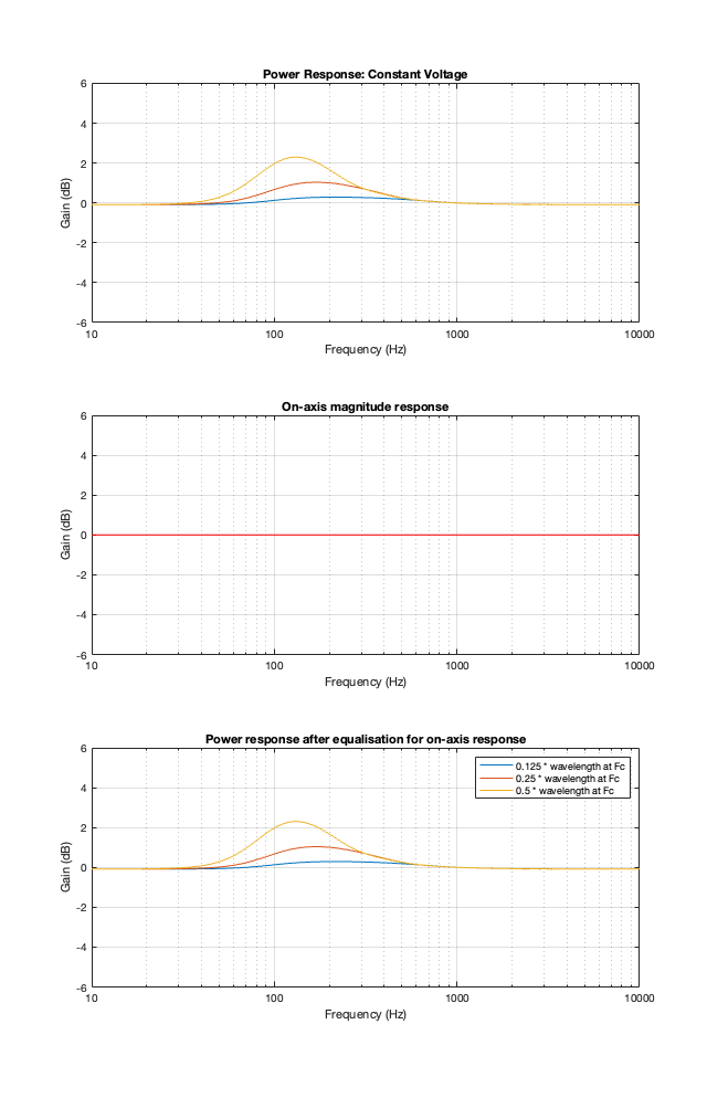
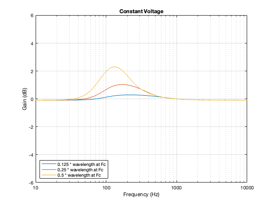
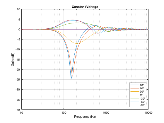
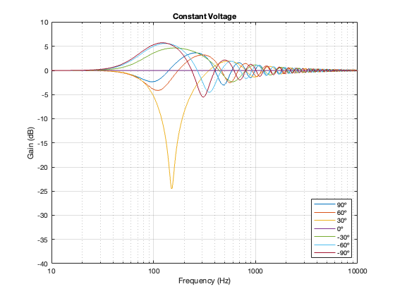
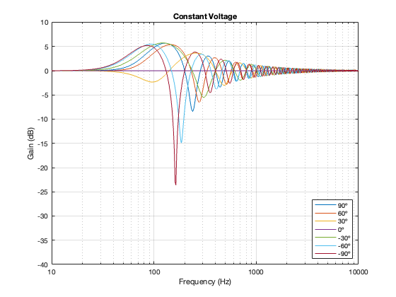
- One version of a Constant Voltage design
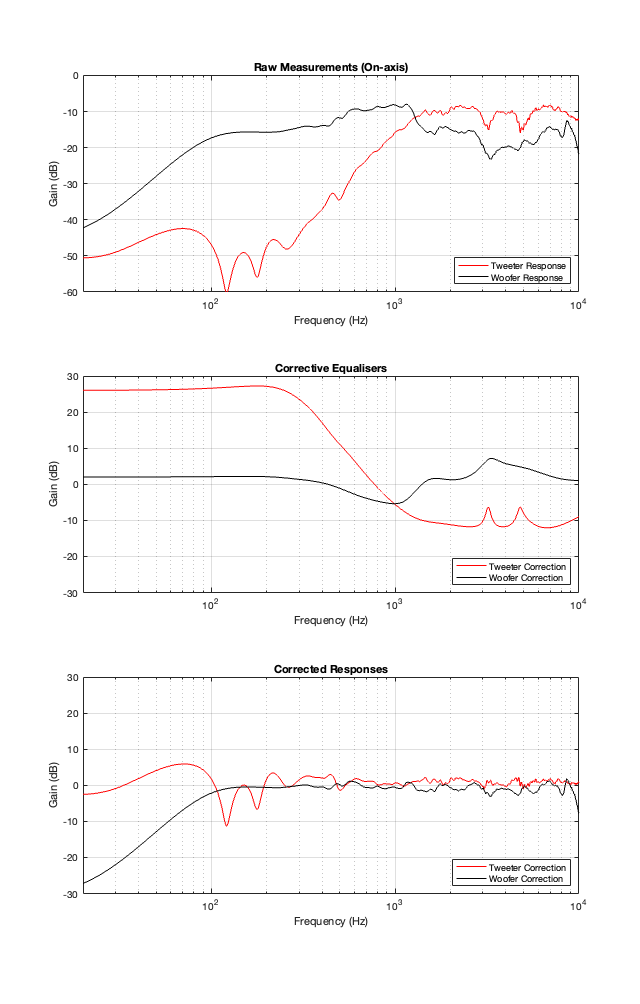
These have been interesting because they’re popular designs, and they are implementable using either analogue circuitry or digital signal processing (DSP). So, everything I’ve said so far is independent of whether the processing is analogue or digital. This is even true of all of those equalisers I applied to the two loudspeaker drivers to force them to be flat. Those are easiest to implement with DSP, but I didn’t do anything there that can’t be done with resistors, capacitors, and inductors.
But, the original question was
In passive crossovers, many are phase incoherent,
meaning that the phase shift of one frequency will be different than another frequency.
Do you agree? Am curious how this is dealt with in the active crossover’s of B&O products?
Hopefully, it’s obvious that the answer to the first question is “yes” – sort of… Passive crossovers are not “phase incoherent” – but they do have an effect on the phase response. As I’ve shown, you can think of the end result of a crossover implemented with minimum phase filters as an allpass filter. So there is an effect on the phase response of the loudspeaker. (Yes, the on-axis response of a Constant Phase crossover can result in a flat phase response, so that one might be an exception.)
However, if we leave analogue signal processing behind and go forwards limited to digital signal processing, then we have another option: linear phase filters.
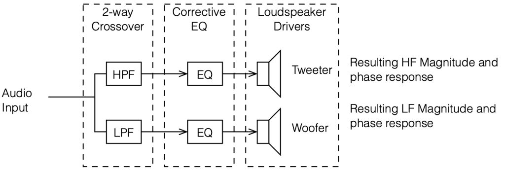
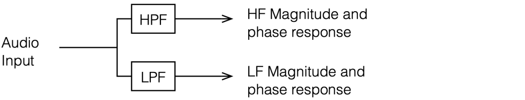
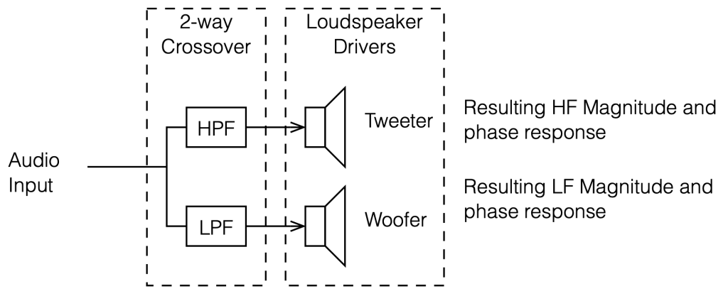
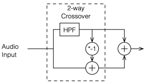
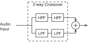
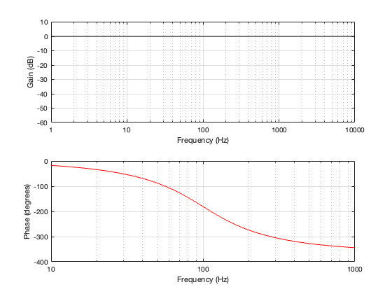
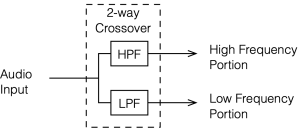
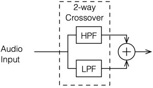
To start, let’s look at our original, simplified method of analysing a crossover, using the block diagrams shown in figures 12.1 and 12.2
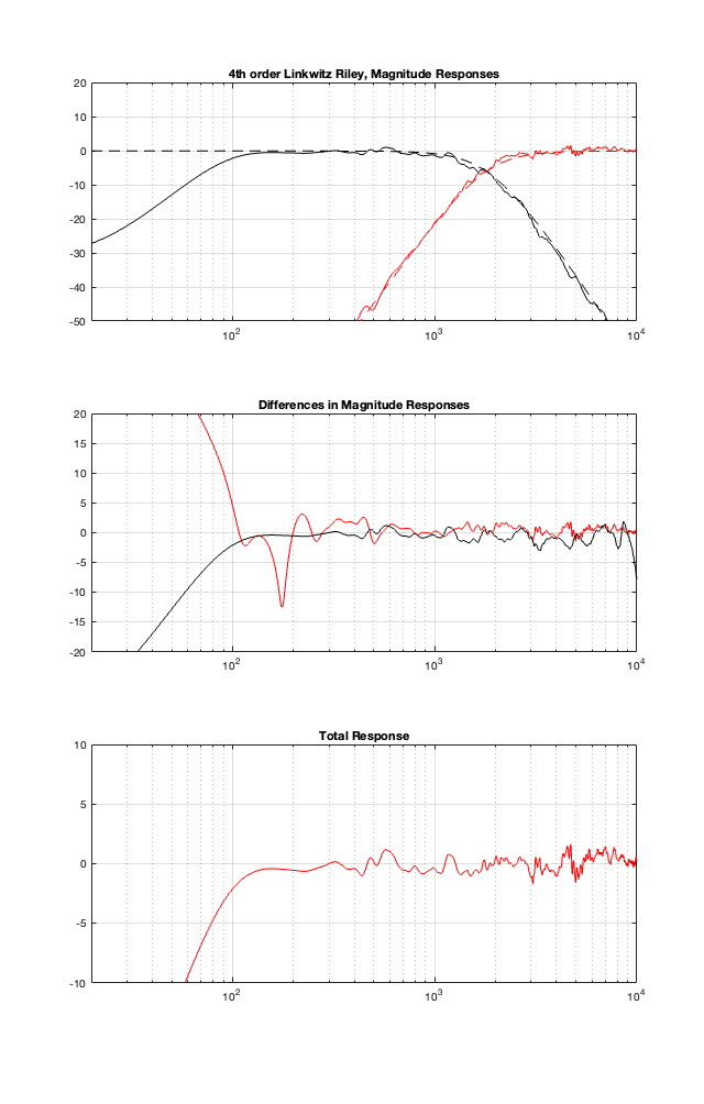
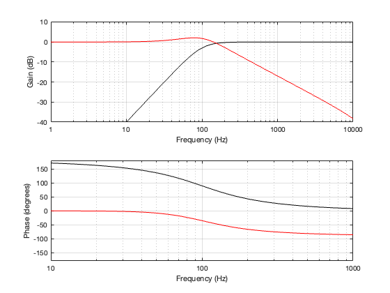
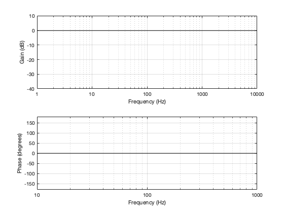
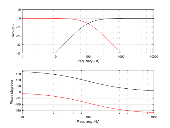
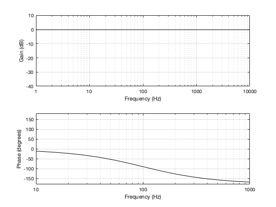
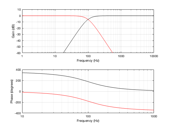
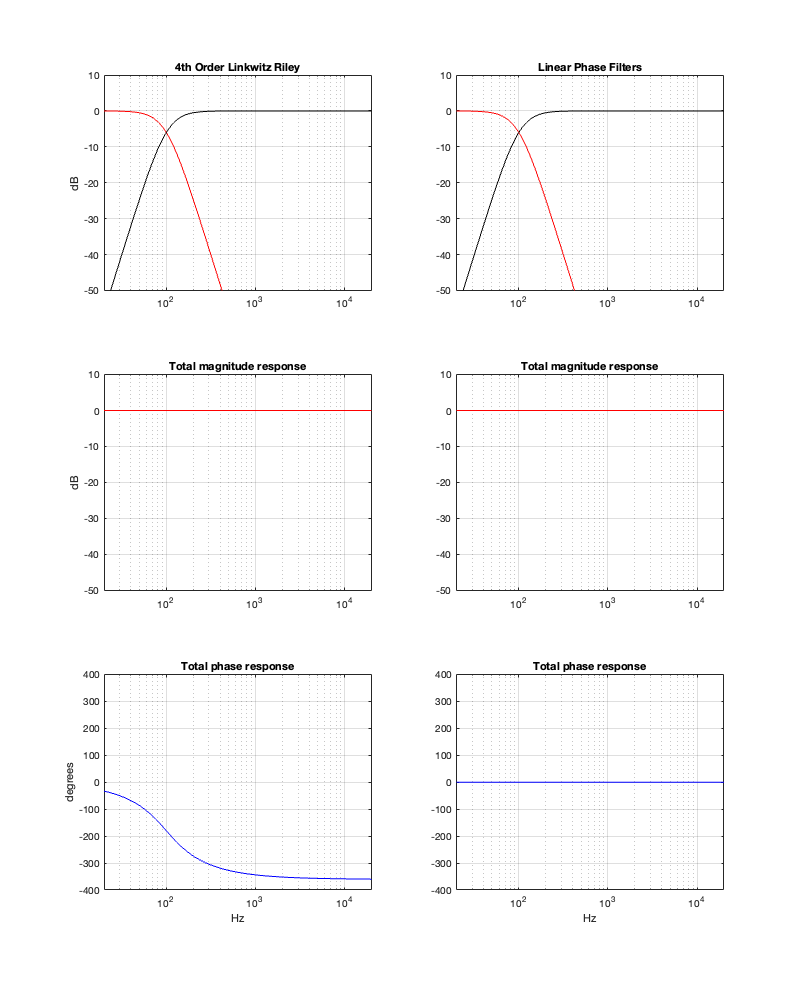
If we use this signal flow and create two crossovers at 1 kHz, one with a 4th-order Linkwitz Riley design (which I’ve already shown) and one with linear phase filters, the responses will look like the ones shown below in Figure 12.3
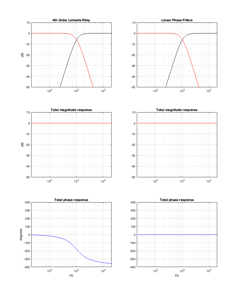
Looking at the magnitude responses, you can see that these two filter designs are identical. However, the phase responses of their total outputs are not. The Linkwitz Riley design behaves like a minimum phase allpass filter, whereas the linear phase design does not.
So, this proves that a linear phase crossover is better, right? Not so fast… We’re not done yet…
Time response
The plots above show the frequency responses (“frequency response” is the combination of the magnitude response and the phase response) of the two designs. However, there is another way to look at the response of a system like a crossover, and that is to analyse how it behaves in time.
If we create a signal that is complete silence, and then a single one-sample-long “click”, we have something called an “impulse”. If we then send that into an audio system (like a crossover, for example), then we can see how it behaves in time – its temporal response. Since this method shows us how the system responds when you send an impulse through it, we call it the “impulse response” of the system.
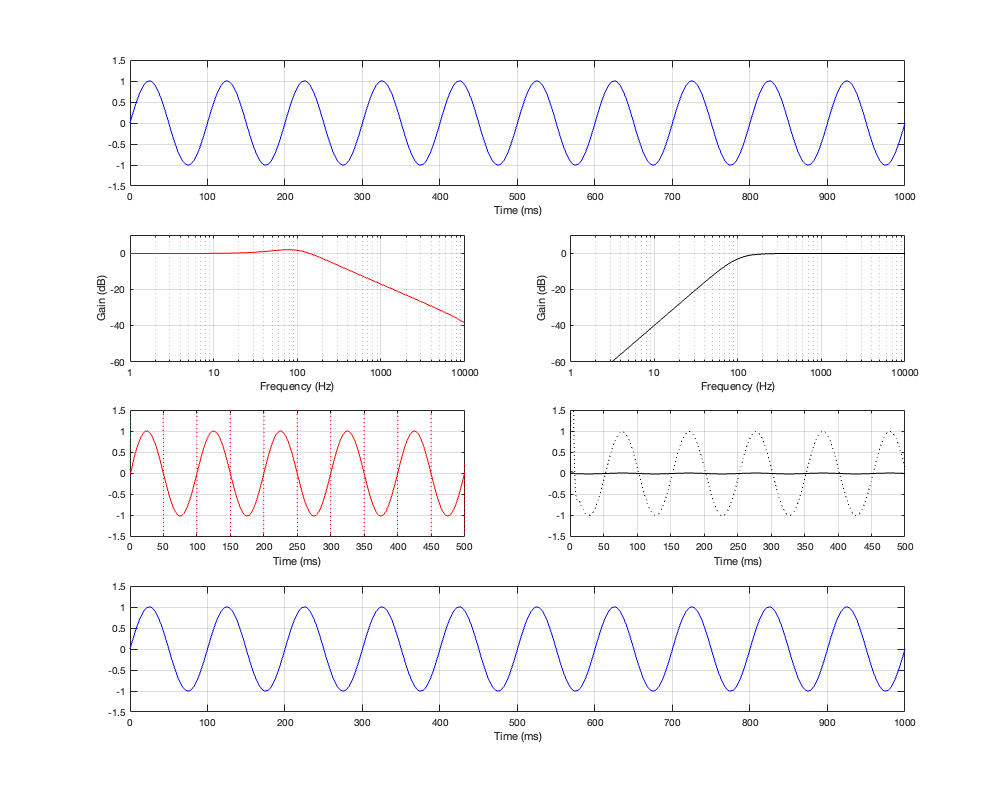
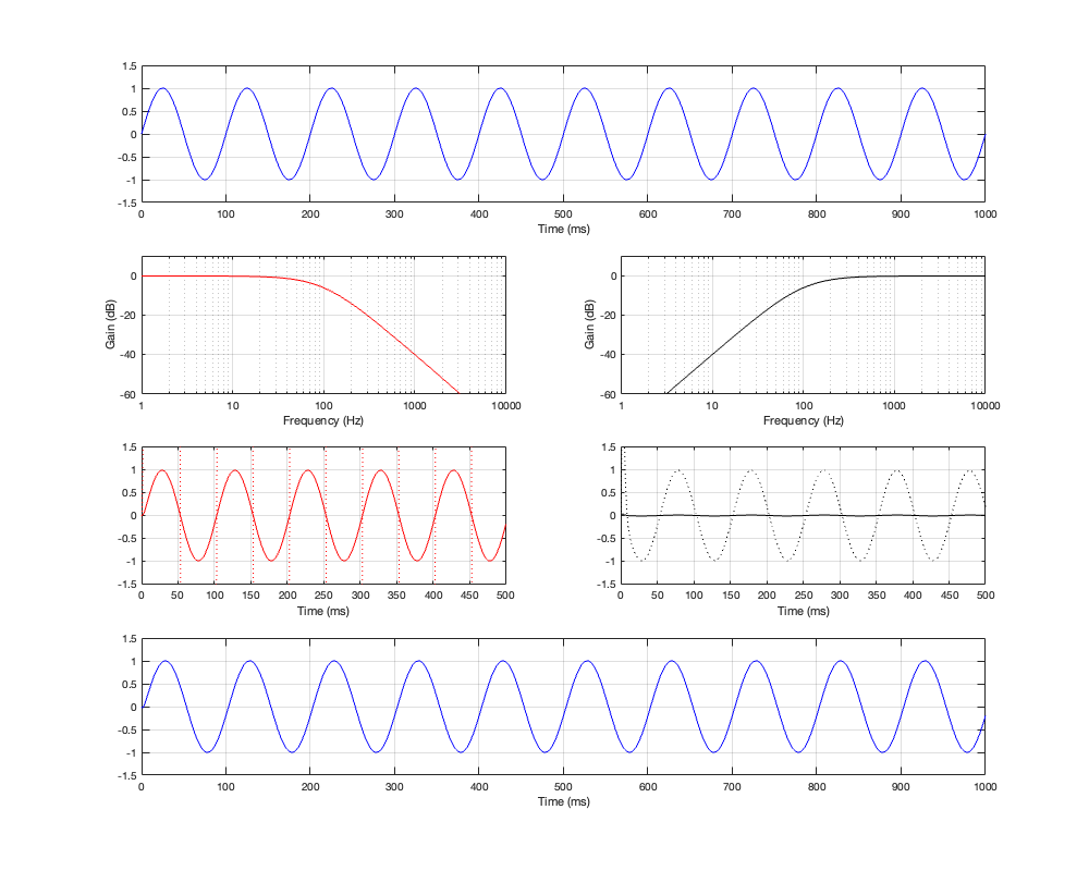
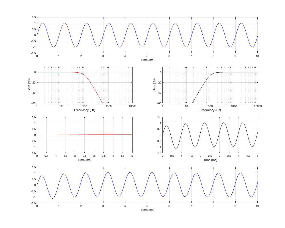
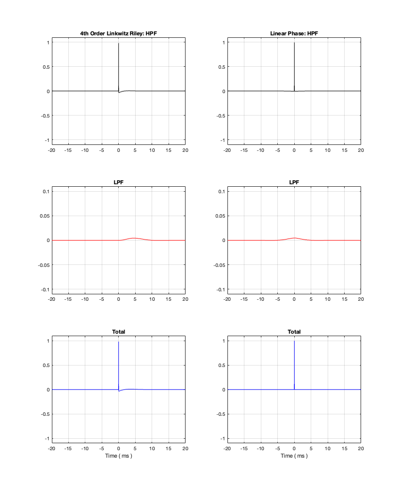
If we measure the impulse responses of our two 1 kHz crossovers, we get the results shown below in Figure 12.4.
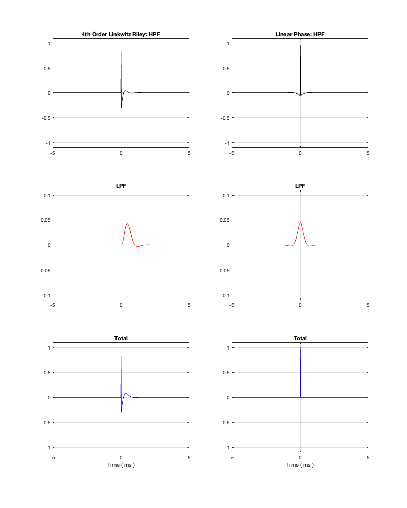
As can be seen in the impulse response plots for the Linkwitz Riley crossover, until the impulse arrives at the input of the filter, the output of the filters are silence. This is the flat line with a constant amplitude of 0 from -5 ms to 0 ms. Then, at time = 0 ms, the impulse hits the input of the crossover, and something happens. The output of the high-pass filter spikes, and the output of the low-pass filter slowly (relatively speaking) starts ramping up. The combined output of the two filters, shown in blue, shows that the output is not a single-sample impulse. It has the characteristic shape of the impulse response of an all-pass filter.
The impulse responses of the high-pass and low-pass outputs of the linear phase crossover are similar-ish… but they have one characteristic that is VERY different. They have an output on the left side of time = 0 ms. One way to look at this is to say that they output a signal before the crossover gets something at its input. This is, of course, impossible: linear phase filters are not time machines.
So, how does this happen? By including a delay in the signal flow. In order to make a linear phase filter, you have to include a delay that starts is as long as is necessary to look after the stuff that you need to do to the signal before that big spike hits. So, if you want to use a linear-phase filter, then the “price” is that the output is going to be late.
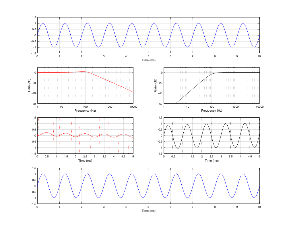
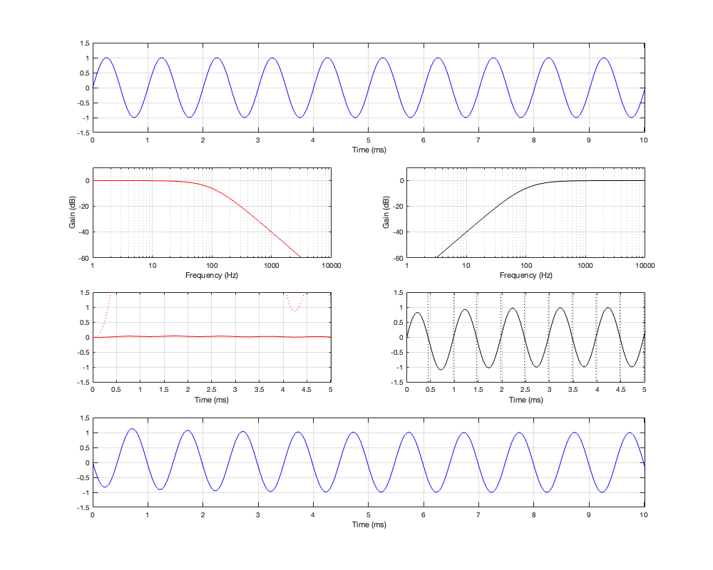
How late? That’s up to you, since it’s a combination of the filter’s frequency and how accurate and precise you want the filter to be. One way to consider this is to look at the plots in Figure 12.4 on a decibel scale. This is shown in Figure 12.5.
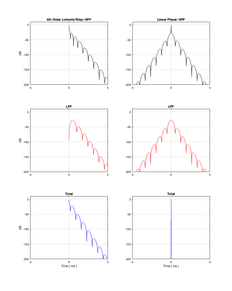
Let’s say, for example, that you have this crossover at 1 kHz and you want to have an impulse response that is accurate down to -100 dB. Looking at HPF and LPF impulse responses for the linear phase crossover, we can see that they drop below -100 dB at about ± 2.4 ms. This means that, if you decide that your threshold of acceptability is about -100 dB (which is pretty good…) then, for a 1 kHz linear phase crossover, you’ll have to include a 2.4 ms delay in your signal path to implement it.
Of course, if you are more picky – say, you want to go down to -200 dB instead, then you’ll have to wait about 4.8 ms (check where the red and black lines get 200 dB down on the left side of the plots.
Notice that I said above that this amount of time – the delay (or as we normally call it: the loudspeakers input-output latency) is also dependent on the frequency of the filters.
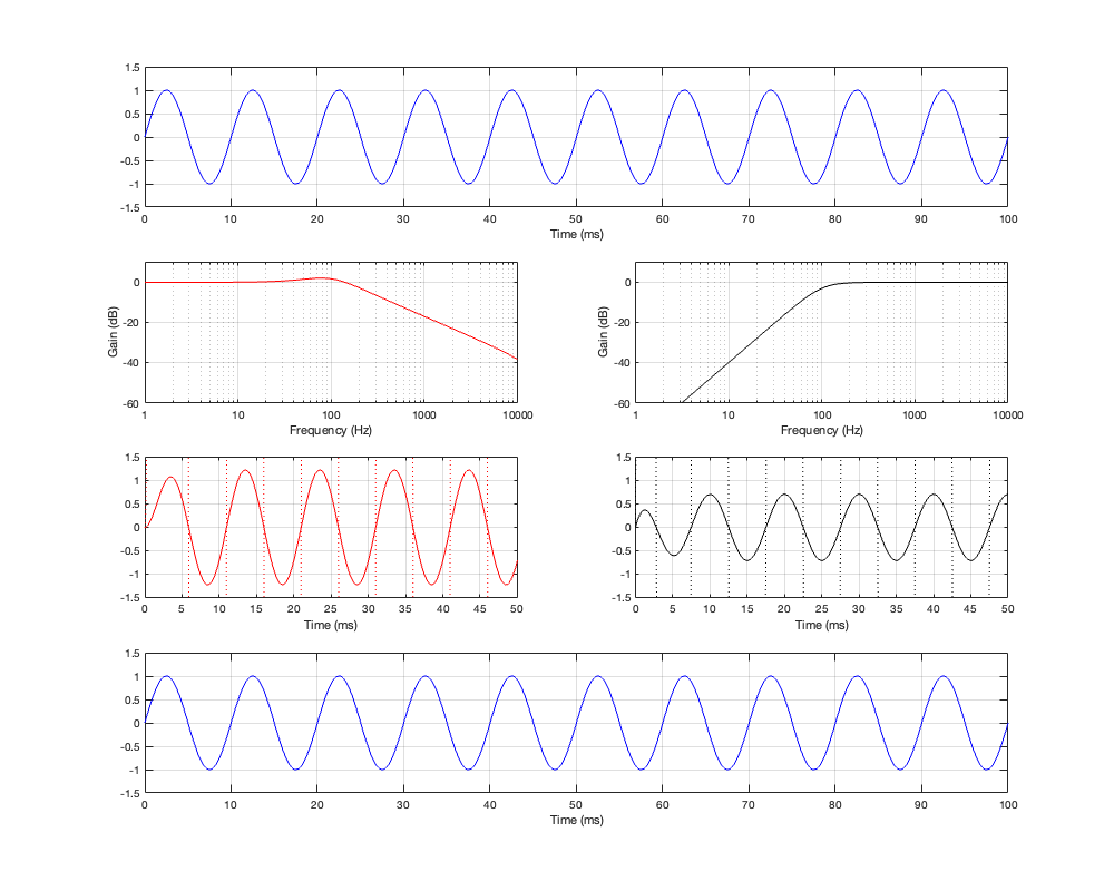
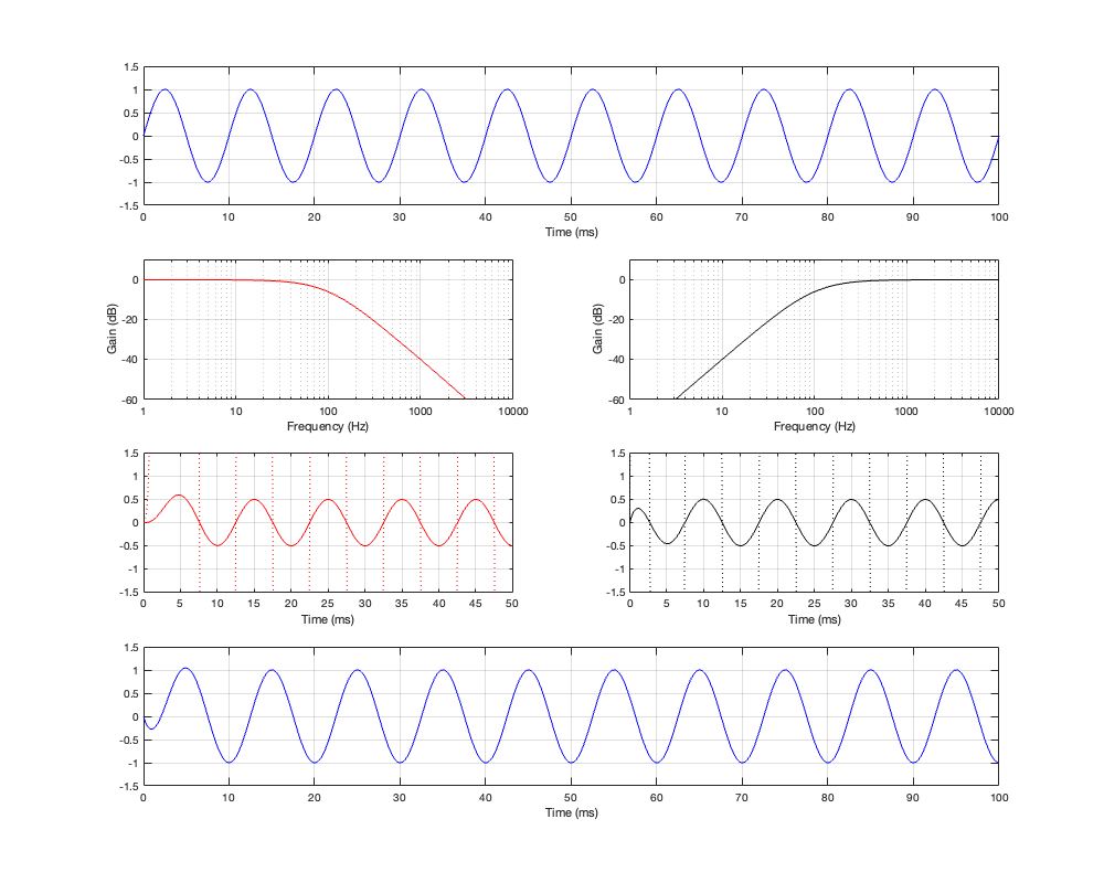
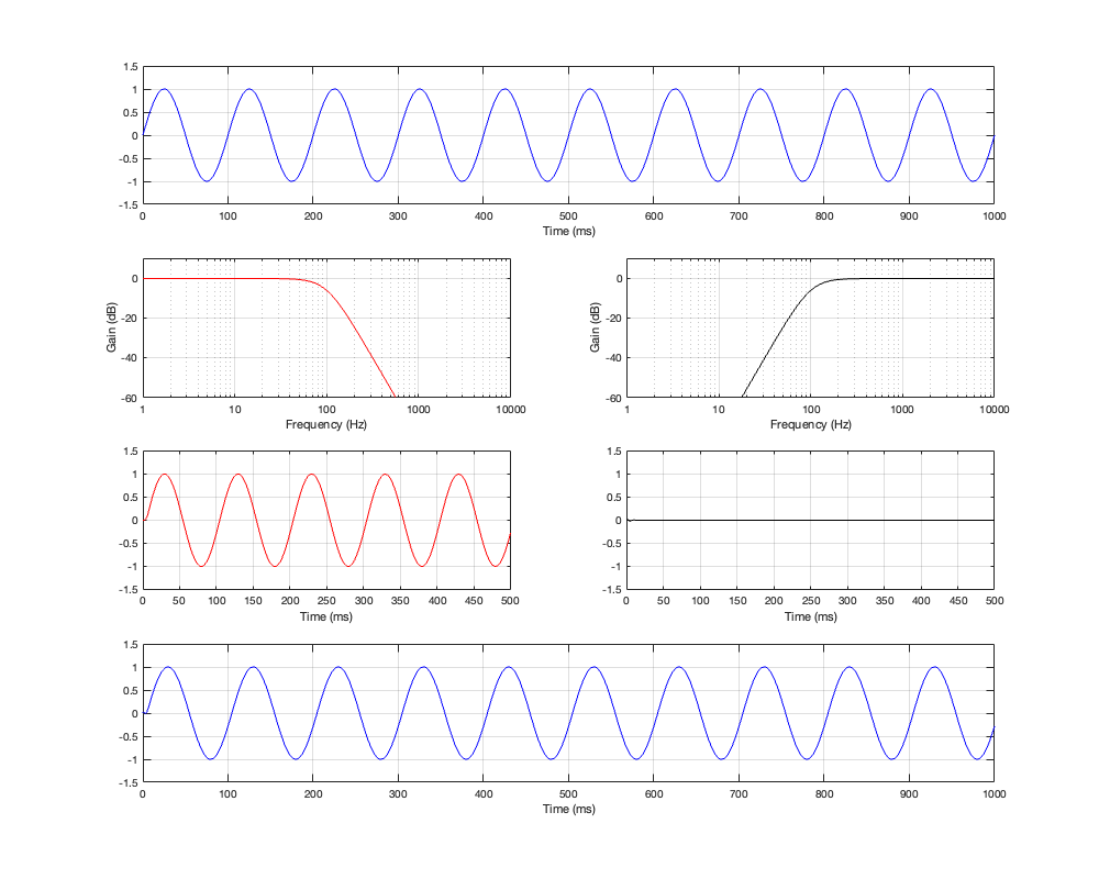
So, let’s look at the same plots for a crossover that is one decade lower: at 100 Hz.
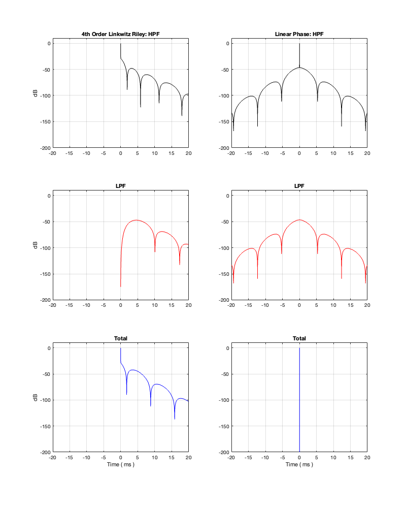
Figures 12.6 to 12.8 show the same plots for at 100 Hz crossover. HOWEVER: notice that the scale of the x-axis has changed to ±20 ms instead of ±5 ms. Also note that, despite me extending that scale by a factor of 4, it’s still not enough to get down 200 dB for the linear phase filters.
You can see there (looking at the red curve on the right of Figure 12.8) that, if you’re going to set -100 dB as your threshold, then you will have to have a latency of about 14 or 15 ms to implement it as a linear phase crossover. (Similar to the 1 kHz version, if you want to go down 200 dB, you’ll need to double this to 28 to 30 ms, which is starting to get close to the acceptable limits for lip-synch with video.)
In the next posting, we’ll look what happens to the magnitude and phase responses if you shorten these impulse responses using a technique called “windowing”.
However, I am NOT going to talk about audibility of a linear phase vs a minimum phase strategy. There are people who love to bang on about ringing and pre-ringing and whether you can hear the “ramp in” of the linear phase filters, or whether the “long” decay time of the minimum phase filters are audible. The best way to stay out of this fight is to not comment on it. If you want to decide whether you can hear these things or not, then you should implement them and have a listen. I can’t tell you what you can or cannot hear. However, if you DO decide to try implementing these for a listening test, make sure that you do it right, that:
- the only difference in the crossovers is what you think it is (If not, you’re not comparing the crossover types in isolation), and
- you are running a blind test (if not you can’t trust your own opinion).