Part 1
Part 2
Part 3
Part 4
Part 5
Part 6
Part 7
Part 8a
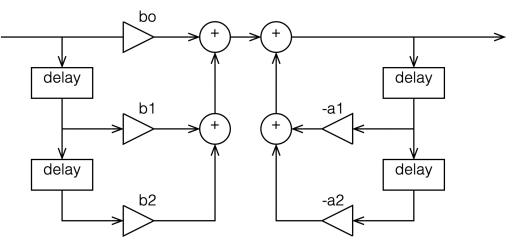
In the previous posting, we left off with this drawing of a biquad filter:
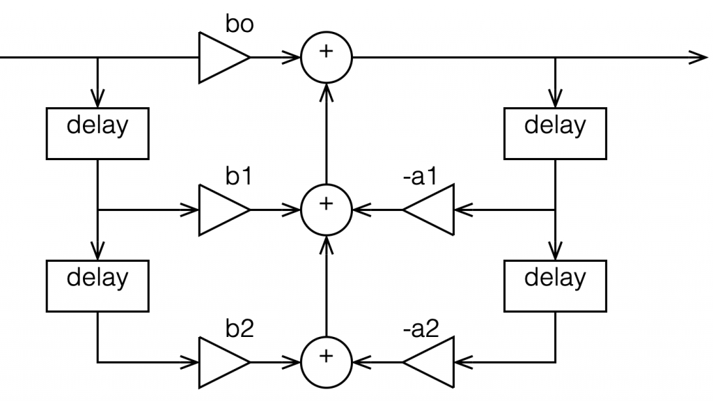
This is not the normal way to draw the signal flow inside a biquad, since it has a little too much information. Normally you see something like this:
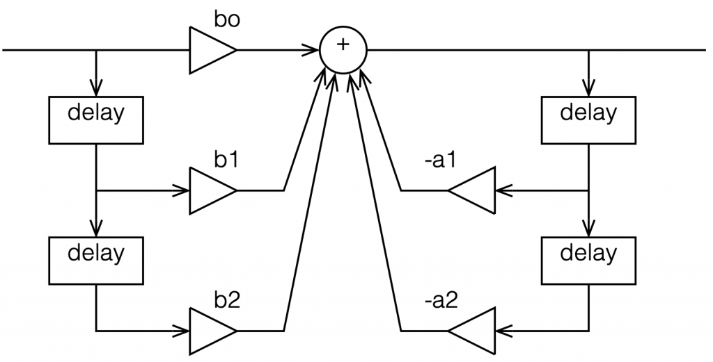
or this:
In the versions I show above, the feed-forward half of the biquad comes first, and its output feeds the start of the feedback portion. It is also possible to reverse these, putting the feedback portion first, like this:
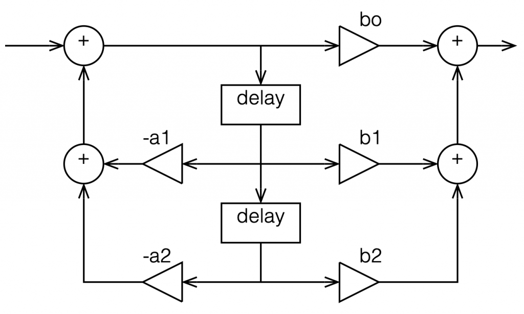
In theory, these different implementations will all result in the same output if you match the gain values. However, in practice, they are not the same, and this difference is where we need to look for this part of the discussion on high res audio.
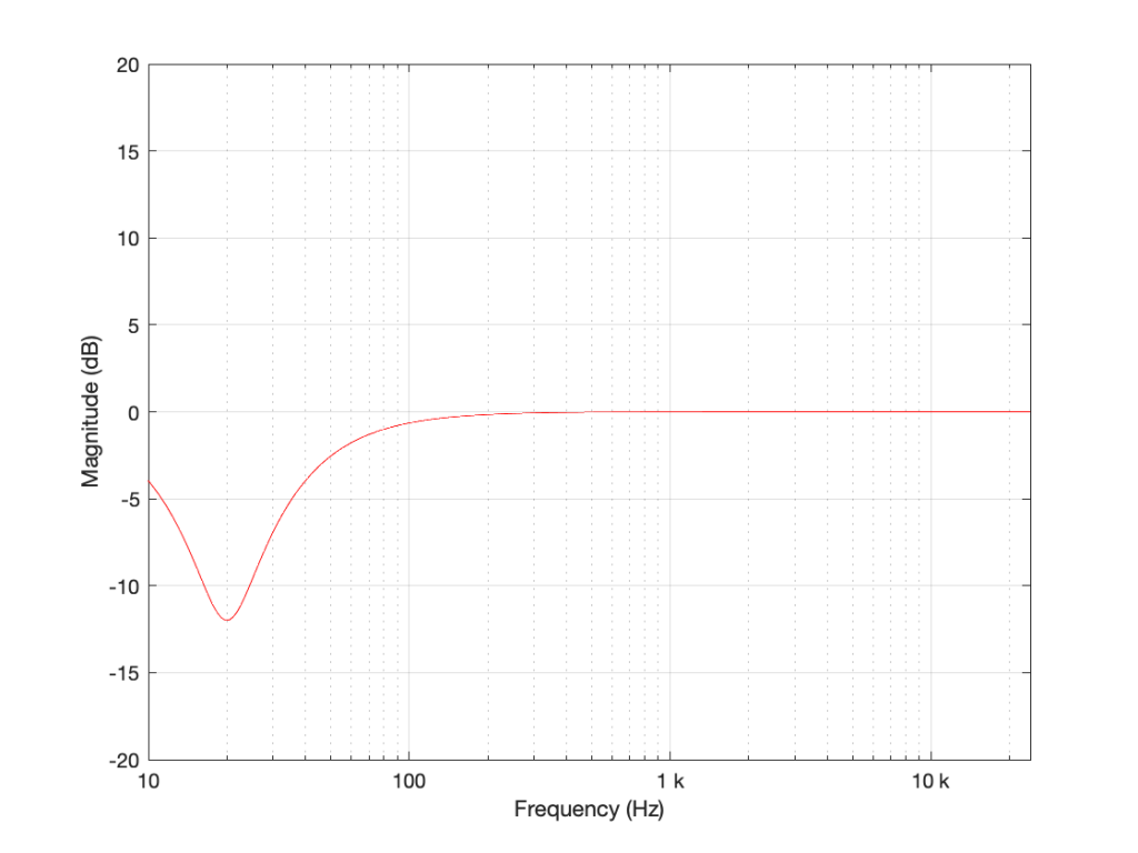
Let’s say I want to make a simple filter that reduces bass in a fairly narrow frequency band. I can use a biquad to do this. For example, if I want a peaking filter that reduces 20 Hz by 12 dB, with a Q of 1, then I get a magnitude response that looks like this:
If I wanted to build this filter using a biquad in a system with a sampling rate of 48 kHz, it would have the following gain coefficients:
b0 = 0.998049357193933
b1 = -1.994783192754608
b2 = 0.996740671594426
a1 = -1.994783192754608
a2 = 0.994790028788359
We’ll also say that my biquad is implemented like the one shown in Figure 1, above… let’s take a look at that signal flow again:
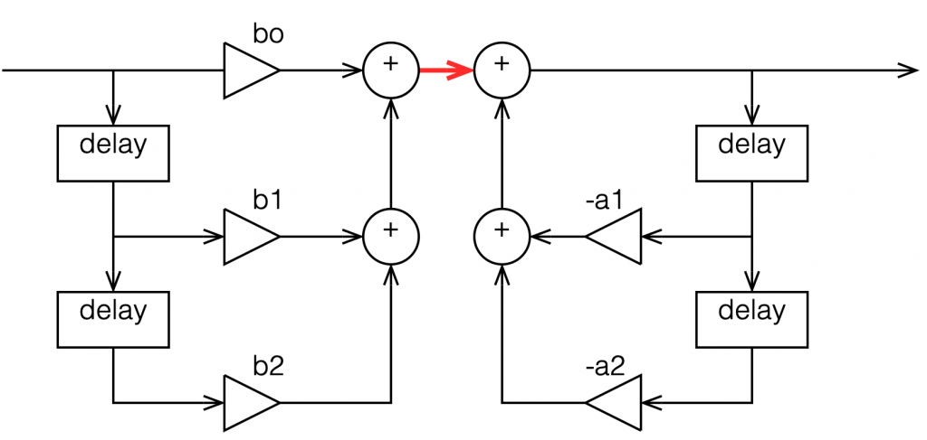
I’ve highlighted a point inside the biquad using a red arrow. Let’s talk about the signal right there, in the middle of the processing…
In the last post, we talked about how, when the signal frequency is very low, a single sample delay has almost the same value at its output as its input, because the phase difference is so small for such a small time. So, let’s start with the (incorrect) assumption that, for those two feed-forward delays at the beginning, their outputs ARE equal to their inputs (because we’re starting with a low frequency). What happens when the input has a value of 1? Then the value at the red arrow is just the sum of the feed forward gains (because I multiplied each of them by 1 and added them together…)
In the case of the filter I described above, this value will be 0.000006836, which is a very small number. Also, if the value coming into the input of the biquad is less than 1, the value at the red arrow will be even smaller! This means that, if you come into the biquad with a low-frequency tone with a level of 0 dB FS, the level at that red arrow will be about -103 dB FS, which is very quiet. The feed-back portion of the biquad, after the red arrow, then has a lot of gain in it to bring the signal level back up towards 0 dB FS again.
So, the issue that we have here is that the FF (Feed Forward) portion of the biquad drops the level A LOT. And the FB portion increases the level A LOT, just to do something like a little 12 dB dip at 20 Hz.
The magnitude of the gains downwards and upwards in those two portions of the biquad are dependent on the parameters of the filter that we’re trying to make, however, we can generalise a little and say that:
- the lower the frequency
OR - the higher the Q,
- then the bigger the gain down and up.
In other words, if you have a really low frequency dip, with a really high Q, then the level of the signal at that red arrow will be really low. REALLY low.
How low can you go?
How low is “REALLY low”? let’s see:
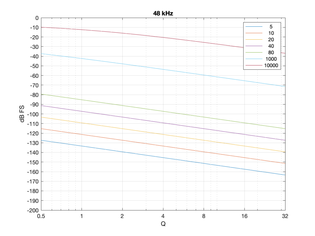
Take a look at Figure 7, which shows some values for one example filter (peaking, Gain = -12 dB, variable Q and Fc, and the test frequency = Fc). Notice that when the Fc is 10 kHz, even at earn Q=32, the signal level at the middle of the biquad is about -38 dB FS or so. However, when the Fc is 20 Hz, it’s -140 dB FS… This is very low.
Now let’s try again at a higher sampling rate: 192 kHz.
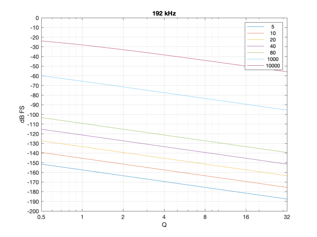
Notice that when we do exactly the same thing running at 192 kHz, the signal levels inside the biquad get much lower. Now for a 20 Hz signal and a Q of 32, the level is around -163 dB FS – a drop of more than 20 dB for 4x the sampling rate.
Why does this happen? It’s because the filter doesn’t “know” that the signal is at 20 Hz. It only knows the relationship between the frequency and the sampling rate. So, in its little world, 20 Hz doesn’t exist. In a system running at 48 kHz, what exists is 20 / 48000 = 0.0004167. This is called the “normalised frequency” where the sampling rate is 1, DC is 0, and everything else is in between. (Note that some textbooks and software say that Nyquist = 1 instead of the sampling rate – but you just need to know what the convention is for the thing you’re reading…) This means that if the sampling rate goes up to 192 kHz, then the normalised frequency for 20 Hz is 20 / 192000 = 0.0001042 (1/4 of the value because the sampling rate was multiplied by 4).
So what?
This is important. If you want to make a low-frequency, high-Q peaking filter in a digital system with a cut of 12 dB, you are forcing the signal to a very low level inside your filter, and then bringing it back up to a normal level again on the way out. If your processing is running with a limited resolution, (e.g. 16-bits, for example) then the signal level can approach or even go below the resolution of your system inside the biquad. This means that, when the signal’s level is raised again on the way out, it’s full of quantisation distortion, and you can’t get rid of it… This is bad.
There are different ways to solve this problem.
- Increase the resolution of your processing internally. For example, even though your input and output might only be running at 16-bits or 24-bits, maybe you need more resolution inside to make the results of the math better – or at least below the limitations of the input and output.
- Change the way the biquad is implemented. For example, if you use the implementation shown in Figure 4 (with the feedback before the feed-forward) instead of the one we used, then you don’t drop the signal level and raise it again, you do the opposite. This avoids your quantisation error problem. However, depending on the system, it might overload and clip the signal inside the biquad instead, so then you just end up with a different kind of distortion instead.
- Reduce your sampling rate to make it closer to your filter’s frequency. The problem I showed above is that the centre frequency of the filter is too far away from the sampling rate. If the sampling rate were lower, then this automatically makes the filter’s centre frequency “higher” in a normalised frequency scale, thus reducing the problem.
- Other, even more clever solutions that I won’t talk about because they’re not as simple.
This means (for example) that if you’re building a subwoofer with digital filtering, and you know for sure that NOTHING will come out of it above, say 1 kHz (just to pick a random number that’s far enough away from the typical 120 Hz that people normally use…) then it would be dumb to do the filtering at 192 kHz. It’s smarter to run its internal sampling rate at 2 kHz (because we only need to go up to 1 kHz; and we’re not considering anything other issues or artefacts in this posting.)
P.S.
For this discussion, I used the specific example of a peaking filter with a gain of -12 dB, and I was varying the Q and the Fc. I was also measuring the level of the signal using a sine wave with a frequency that was the same as Fc in each case. However, the general lesson here about low frequency and high-Q filtering holds for other filter types and implementations as well.