Part 1
Part 2
Part 3
Part 4
Part 5
Part 6
Part 7

Almost every audio system has filters or equalisers in it for some reason or another. Originally, equalisers were named that because they were put in on long-distance telephone lines to make the balance of the frequency content more equal. Nowadays, we use equalisers to do things like add bass, or to add more bass.

In the “old days” audio filters were made by building circuits with resistors, capacitors, and inductors: if you choose the relationships between the values of these devices correctly, you can affect the magnitude response as you choose. The problem was production tolerances: if you take two resistors out of the package, and both are supposed to have the same resistance – they’ll be close, but they won’t be identical.

One of the great things about audio filters implemented in a digital system is that you don’t need to worry about variations as a result of production differences. Since digital filters are “just math”, you put the same equation in every device, and you get the same answer for the same input every time. (In the same way that, if I have two calculators on my desk, and I put “2 x 3″ into both of them, and press”=”, I’ll get the same answer on both devices.)

So, to start, let’s talk a little about how a digital filter works. Generally speaking, digital filters work by taking an audio signal, delaying it, changing the level, and adding the result back to the signal itself. Let’s take a simple example, shown in Figure 1.

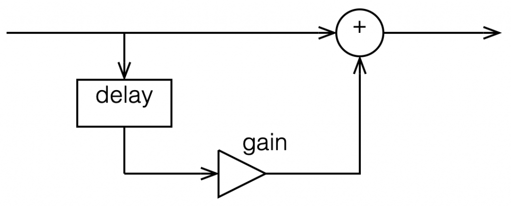
Let’s say that, to start, we make the gain in that signal flow = 1, and set the delay to equal 1 sample. In this case:

• At a very low frequency, the output of the delay has almost exactly the same value as its input (because 1 sample is a phase difference of almost 0º at a low frequency). When you add a signal to (nearly) itself, you get twice the output – a gain of 6 dB.
• As the frequency of the input goes higher and higher, the delay (of 1 sample) is more and more significant, and therefore its output value gets more and more different from its input value.
• When the input signal’s frequency is 1/2 of the sampling rate, then a delay of 1 sample is equal to a 90º phase shift. When you add a sine wave to itself with a “delay” (actually a “phase shift”) of 90º, the result is a magnitude that is 3 dB higher than the original.
• When the input signal’s frequency is 1/3 of the sampling rate, then a delay of 1 sample is equal to a 120º phase shift. When you add a sine wave to itself with a “delay” (actually a “phase shift”) of 120º, there’s no change in the magnitude (the level).
• When the frequency is 1/2 the sampling rate, then each consecutive sample is 180º out of phase with the previous one, so the sum of the delay and the signal results in complete cancellation, and you get no output at all.

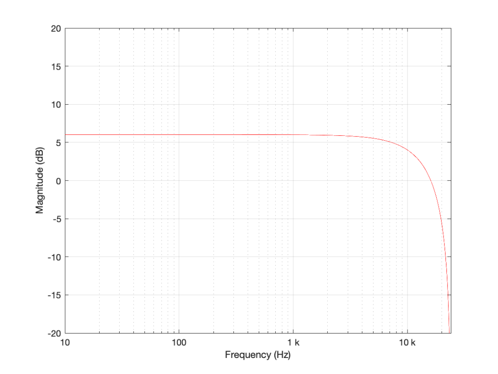
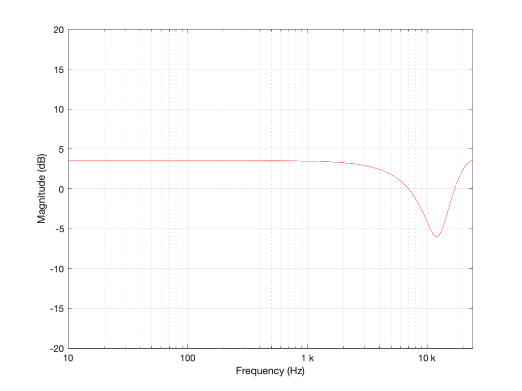
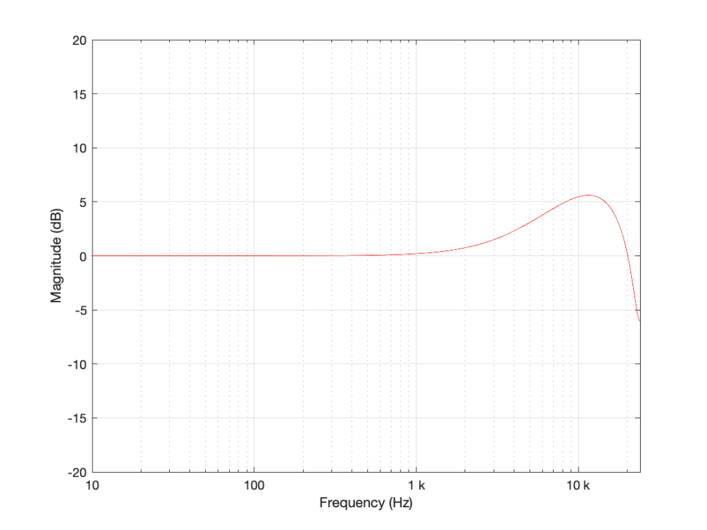
An example of the magnitude response plot of this is shown below in Figure 2.

If we reduce the gain to, say 0.5, then the effect of adding the delayed signal is reduced. The overall shape of the magnitude response is the same, it’s just less, as shown in Figure 3.

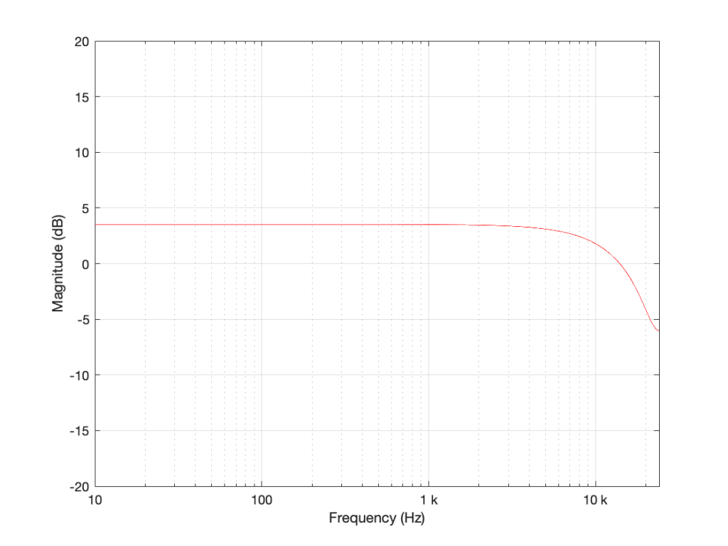
Notice in Figure 3 that the boost in the low end is less, and the dip in the high end is also less than in Figure 2. So, by adjusting the gain on the delayed signal that’s added to the original signal, we can adjust how much this filter is affecting the signal.

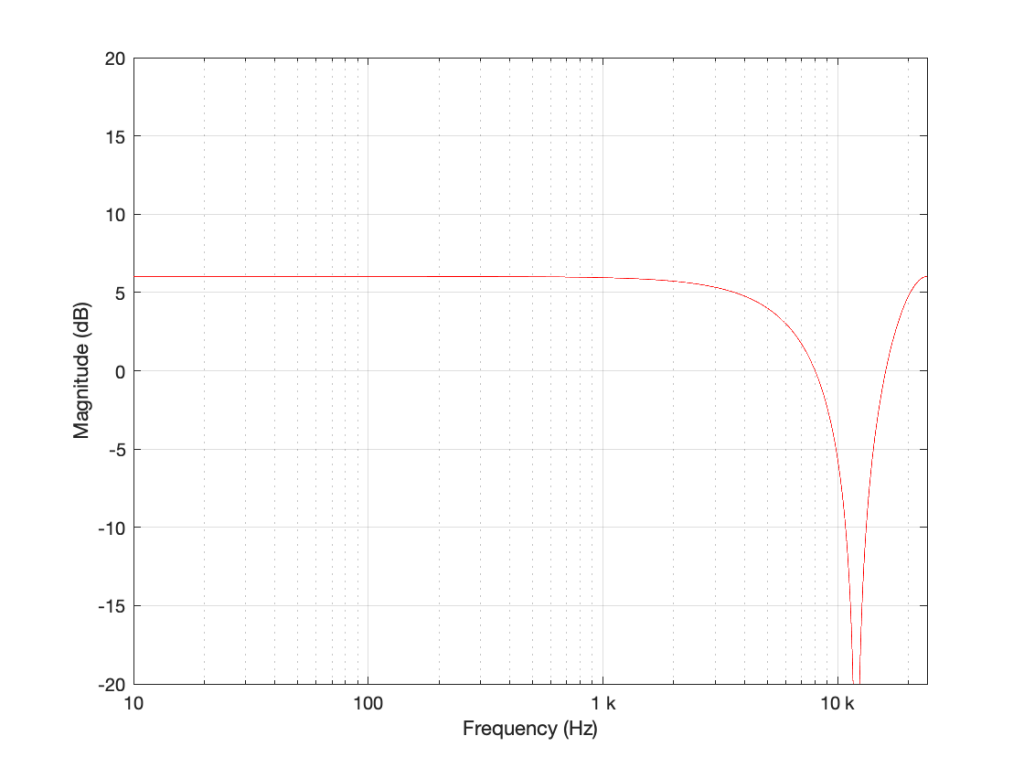
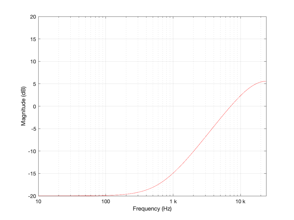
What happens when we change the delay? If we make it 2 samples instead of 1, then the phase difference between the output and the input of the delay will be bigger for a given frequency. This also means that the delay will be equivalent to a 180º phase shift at 1/4 Fs (instead of 1/2). Also, at 1/2 Fs, the delay will be equivalent to a 360º phase shift, so the signal adds constructively, just like it does in the low frequencies. So, the resulting magnitude response will look like Figure 4.

Again, if we reduce the gain, we reduce the effect of the filter, as can be seen in Figure 5.

Now let’s make things a little more complicated. We can add another delay and another gain to get a little more control of things.

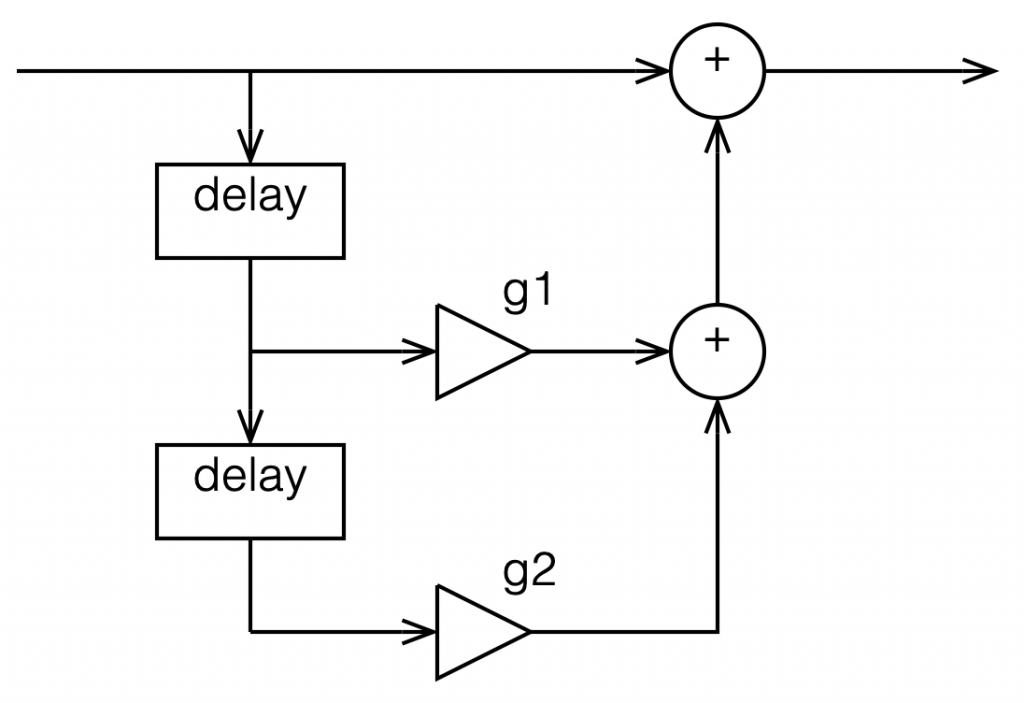
I’m not going to get very detailed about this – but if each of those delays is just one sample long, and we only play with the gains g1 and g2, we can start getting some nice control over the response of this filter. Below are some examples of the results we can get with just this filter, playing with the gains.

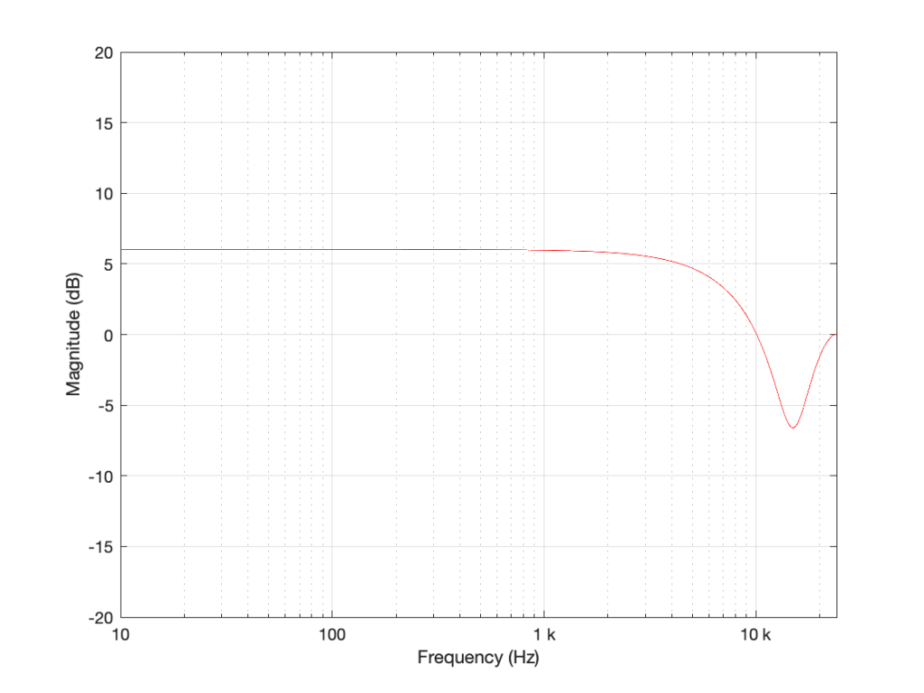
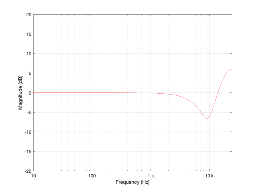
So, as you can see, all I need to do is to play with those two gains to get some nice control over the magnitude response.

Up to now, everything I’ve done is to add a delayed copy of the input to itself. This is what is known as a “feed-forward” design because (as you can see in Figures 1 and 6) I’m feeding the signal forwards in the flow to be added to itself. However, if there’s a “feed-forward”, it must be because we want to distinguish it from a “feed-back” design.

This is a filter where we delay the output (instead of the input) multiply that by a gain, and add it to the signal, as shown in Figure 11.

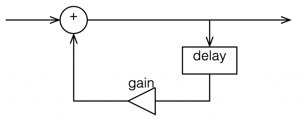
This feedback means that, if the gain is not equal to zero, once a signal gets into the input, the output will last forever. This is why this kind of filter is called an infinite impulse response filter (or IIR filter): because if an impulse (a short spike) gets into it, there will be a signal at the output until the end of time (theoretically, at least…).

And, yes… the output of a filter without a feedback loop will eventually stop, which means it’s a finite impulse response filter (or FIR). Stop the input signal, wait for the last delay to send its signal through, and the output stops.

So what?

Most filters in most digital audio devices are built on a combination of these two types of designs. If you take Figure 6 and you combine it with an extended version of Figure 11 (with two delays instead of just one) you get Figure 12:

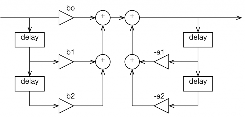
This combination of FIR and IIR filters is a powerful little tool that forms the heart of almost every digital audio filter in the world. (yes, there are exceptions, but they’re definitely exceptions…). There are different ways to implement it (for example, you could put the IIR before the FIR, or you could re-draw it to share the delays) but the result is the same.

This little tool is what we call a “biquadratic filter” or “biquad” for short. (The reason it’s called that is that the effect it has on the signal (its “transfer function”) can be mathematically expressed as the ratio of two quadratic equations – but I will not say anything more about that.) Whenever developers are building a new digital audio device like a loudspeaker or a pair of headphones or a car audio system, it’s common in the early meetings to hear someone ask “how many biquads will we need?” which is a way of asking “how much processing power and memory will we need?” (In the same way that I can measure prices in pizzas, or when I was a kid I would ask “how many more Sesame Streets until we’re there?”)

At this point, you may be asking why I’ve gone through all of this, since I haven’t said anything about high resolution audio. The reason is that, in the next posting, we’ll look at what’s going on inside that biquad when you use it to do filtering – and how that changes, not only with the filters you’re building, but how they relate to the sampling rate and the bit depth…