This week, I was testing a device that required that I look WAY down into the floor caused by the noise+distortion artefacts in the presence of a signal.

One trick to do this is to play a sinusoidal wave through the system and do an FFT of the output. However, as I described in this posting a long time ago, there is an interaction between the frequency you choose and the behaviour of an FFT on a digital signal (yes… I know it’s really a DFT – but let’s not be pedantic…)

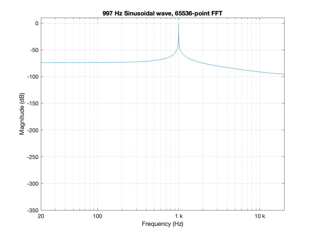
For example, if I do a 65536-point FFT on a 997 Hz sine tone in a 48 kHz sampling rate (with all the floating point precision I have available…) I get a magnitude response that looks like this:

Obviously, this is NOT the magnitude response of a sinusoidal wave. The “skirts” on either side of 997 Hz are artefacts caused by the fact that I’m using a rectangular window, and the sine wave’s last sample does not line up perfectly with its first when the FFT “wraps” it around to meet itself (read this leading up to Figure 10 for an explanation). That sharp discontinuity causes the extra energy in the other frequency bins as shown above.

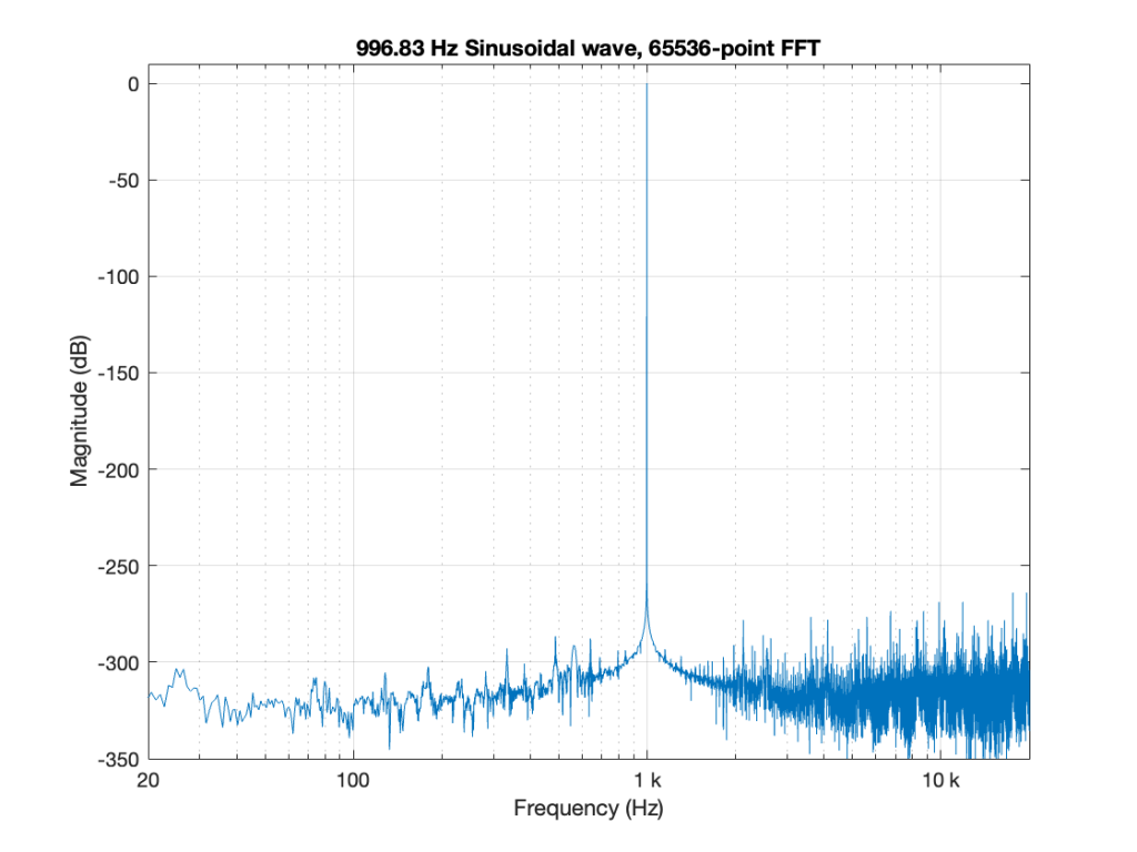
If, however, I find out the frequency of the closest FFT bin, and make my sine wave THAT frequency instead, THEN I do an FFT and look at the magnitude response, it looks like Figure 2.

Notice that this is not a 997 Hz tone, but a 996.8261718750000 Hz tone instead.

Now the “noise floor” that you see there is the error in my sine wave caused by the precision of my calculator (Matlab). -300 dB is VERY low, and gives me plenty of room to see the errors in the thing that I might be testing (assuming that I can actually get that signal out to my Device Under Test or “DUT” and back in again from it).

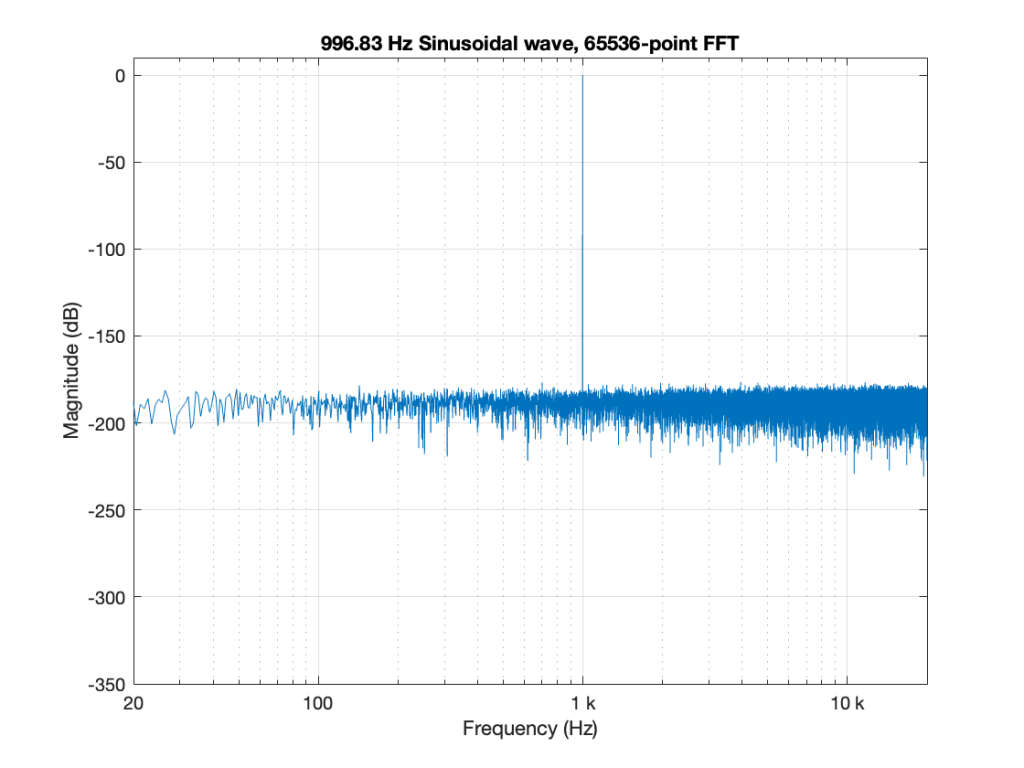
Let’s say I were to represent the same sine wave using a 24-bit LPCM signal that has been correctly dithered with TPDF dither, and THEN I do the FFT and calculate the magnitude response. That would look like Figure 3.

Now, the energy at all the frequencies other than 996.8-ish Hz is the energy in the noise floor generated by the dither. (If you’re wondering why it’s almost 200 dB down, and not 141 dB down (6*24-3), it’s because the total energy in all those FFT bins add up to a noise floor that’s 141 dB below the sine tone.)

Okay. All of those plots show things that I’ve seen before – and are things that I would expect to see when measuring a device.

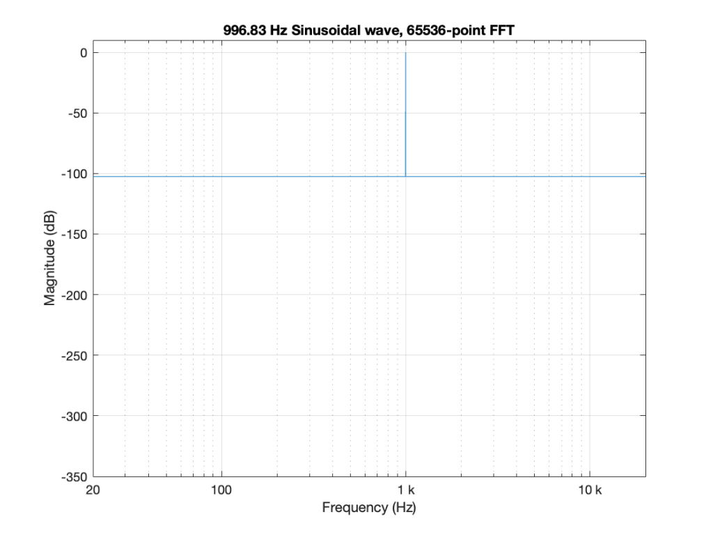
But then, this week, I did a measurement that produced the magnitude response shown in Figure 4.

This is NOT something I’ve seen before, so it raised one of my two eyebrows. In retrospect, I should have known what would cause this, but at the time, I was very confused. It’s not a noise floor because it’s too flat. It’s not distortion because it doesn’t have harmonics. So what is it?

The answer is actually really simple.

• The sine tone is visible as the spike in the magnitude plot, just like in all the others.
• The flat horizontal line is the result of a single-sample click that happened sometime in the 65536 samples that I used to do the FFT.

The sum (or mix) of the sine + click results in the magnitude response plot you see above. If you’re looking at the signal itself, it just means that one of the 65536 samples has an error, and isn’t sitting on the sine curve. I’ve shown an example of this in Figure 5.

The greater the error of that one sample value, the higher the floor in Figure 4.

Of course, for these plots, I simulated everything in Matlab. However, the actual result was even more interesting / confusing, since the DUT didn’t have a flat magnitude response. So, instead of a nice, horizontal line like the one I’ve shown in Figure 4, I could see something like the response of the system as well, but I’ll stay away from the details of that to keep things simple here.