In my previous posting, I mentioned that I was using a tone at or around 997 Hz to test my signal. In truth, only one of the plots I showed there actually used 997 Hz – but that doesn’t really matter.

The question that I’ll talk about in this posting is “why did I prefer to use 997 Hz instead of 1 kHz as my target frequency?” (I didn’t just randomly choose 997 Hz – it’s a common number that’s often used by people in the audio industry.)

The answer to that question has to do with some considerations on how digital audio equipment and software is tested.

Let’s start by talking a little about how a signal gets a PCM (Pulse-Code Modulation) representation in the digital domain. Note that this is the VERY basic explanation – I’m leaving out a lot of steps here…

We’ll start with a signal like the portion of a sine wave shown in Figure 1.

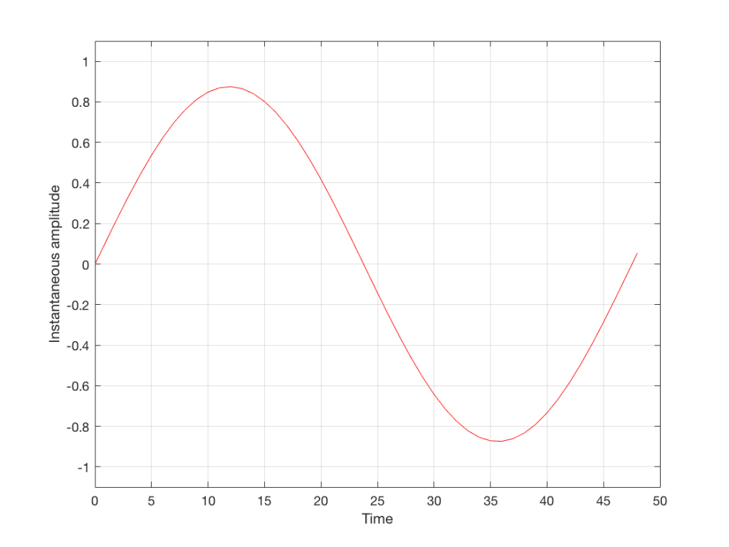
This signal is continuous – meaning that we can zoom in infinitely and still get a smooth curve – both in terms of time, and amplitude.

We then take that signal and measure its amplitude every time a clock ticks – and regular intervals. This is represented by the red dots in Figure 2. (I just left out a whole lot of information about anti-aliasing filters, but it doesn’t matter for the purposes of this discussion…)

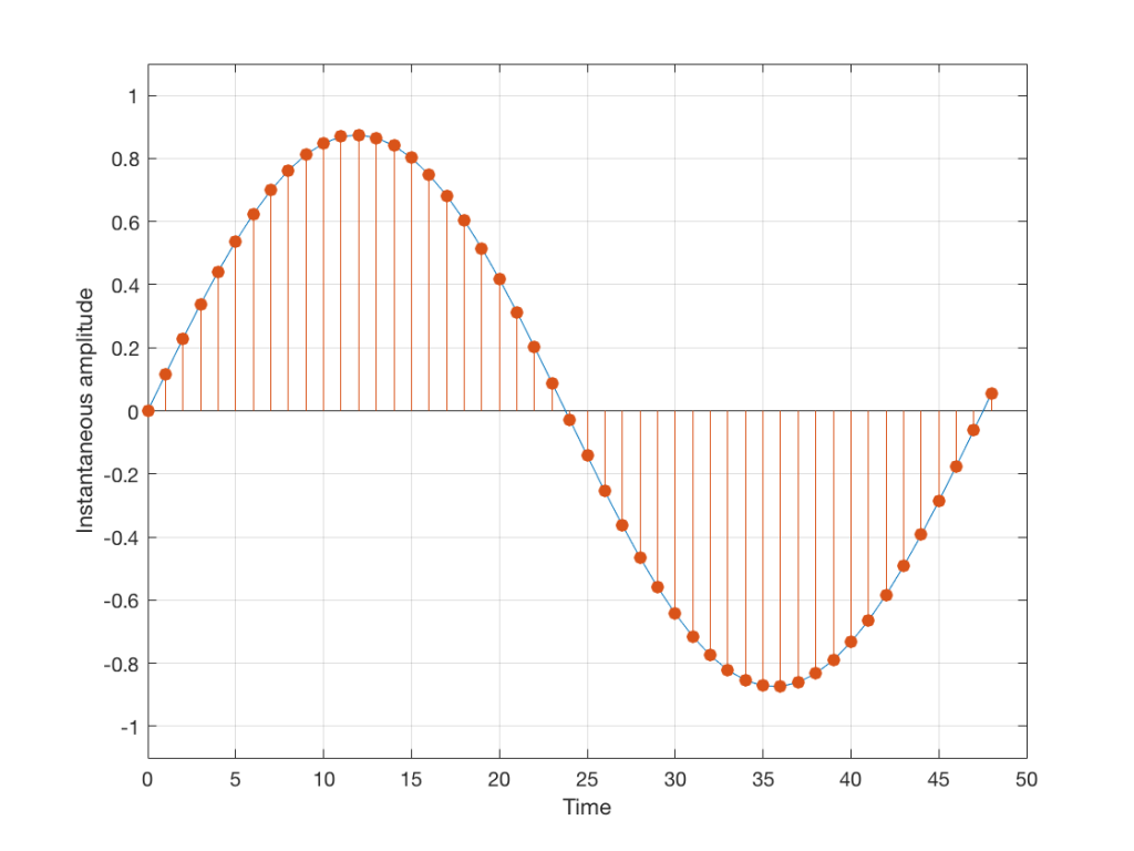
So, in Figure 2 we have a representation of a sinusoidal wave that has been “sampled” – a word that means “measured at regular time intervals. We are grabbing a “sample” or a “measurement” of the amplitude of the signal.

The problem is that the “ruler” we use to measure those values doesn’t have infinite resolution – just like the ruler that you would use to measure the length of something. If your ruler has lines only as fine as millimetres or 1/16th of an inch, then you cannot measure something accurately to the micrometer or to 1/64th of an inch. So, you “round off” your measurement to the nearest value on the ruler.

We do the same with audio – we have a finite number of values that we can store or transmit to represent the instantaneous amplitude of the signal, so we have to round off or “quantise” the values to the nearest value that we have. The result looks something like Figure 3:

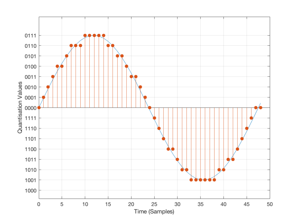
I’ve shown the quantisation values on the left (the Y-axis) as binary values. As you can see there, we have a 4-bit signal which gives us a total of 2^4 = 16 possible quantisation values for storing the signal’s amplitude at each sample.

If you’re really paying attention, you’ll notice that there are one fewer positive values than negative values, since one of the positive values is taken to represent the “0” line. This is why, when I made my original signal, I didn’t scale  it all the way up to ±1 – just to keep things smooth in the explanations. If you aren’t paying that much attention, and you didn’t notice this – then please have a look, since it will come up again later…

Normally, of course, we store audio signals with a LOT more bits than this – a CD uses 16-bit resolution, which gives us a total of 65536 possible quantisation levels (2^16). Other systems use a different number of bits – either fewer or more, depending.

At this point, it should be pretty clear that you have a finite number of samples (or measurements) per second (typically 44100 samples per second (or 44.1 kHz), if it’s a CD, although 48000 samples per second (48 kHz) is also a pretty common number – other systems use other values for this.)

So, if we look at a CD, we have 44100 samples per second, and  65536 possible quantisation values to choose from for each sample (because it’s a 44.1 kHz, 16-bit system). Notice that we have more quantisation values than samples per second…

Now, let’s say that we want to test a piece of digital audio gear, and one of the tests that we wanted to perform was to ensure that all possible quantisation values are working properly (whatever that means). Let’s also say that the gear has only 4 bits of resolution and is running at a sampling rate o 48 kHz, to start. One way to test any audio gear is to feed in a sine tone and to see what comes out. So, we’ll do that, using a 1 kHz sine tone. The result looks like Figure 4, below.

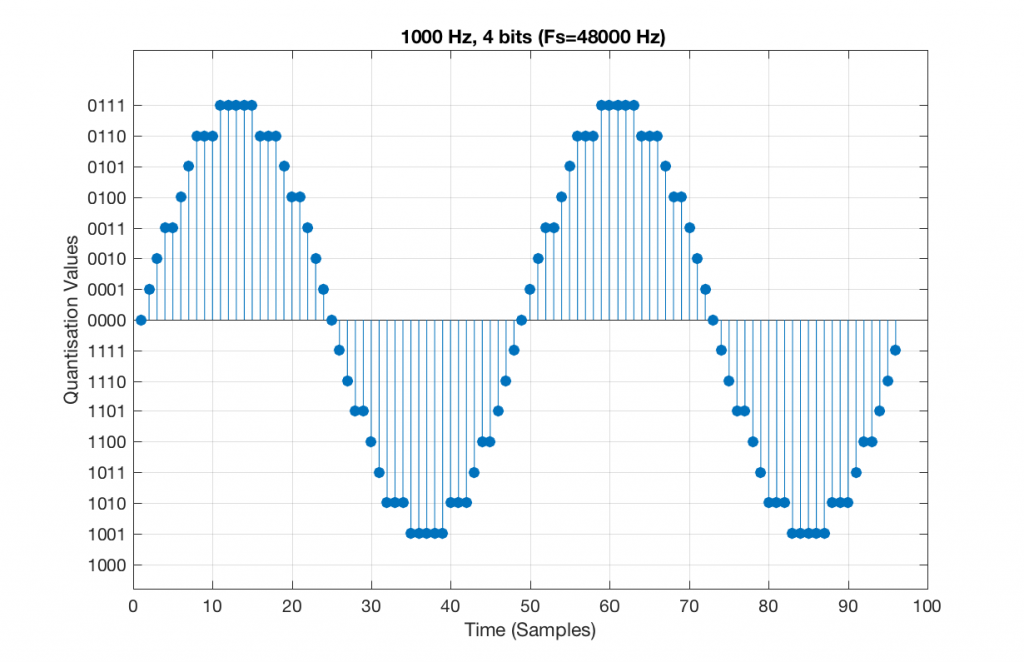
There are two things to notice about that signal in Figure 5:

• The first is that all possible quantisation values are used at least once – except for the very bottom one – but that last one is my fault, caused by the scaling of the sine wave, and the fact that it is symmetrical.
• The second is that the wave is perfectly periodic – meaning that it repeats itself over and over and over… There are two cycles of the waveform shown in the plot, and if you count the dots, you’ll see that the two are identical. This second point is the one that will be important to understand as we go further. The reason this exact repetition happens is because the frequency of the sine tone (1000 Hz) is an integer divisor of the sampling rate (48000 Hz). In other words, 48000 / 1000 = 48 – not a weird number like 48.3.

Let’s take that same signal (1 kHz in a 4-bit, 48 kHz PCM system) and we’ll count the number of times each sample value occurs after 1 second (or in a time of 48000 samples). We can then plot these values as is shown in Figure 6, which is a kind of plot called a “histogram”.

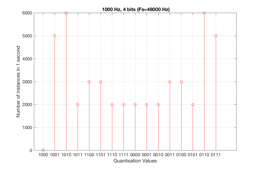
As can be seen in Figure 6, the bottom quantisation value (1000) is never used – but apart from that one, all others are.

Let’s do the same thing, but with a 4-bit, 44.1 kHz system instead. The results of this are shown below in Figure 7 and 8.

 

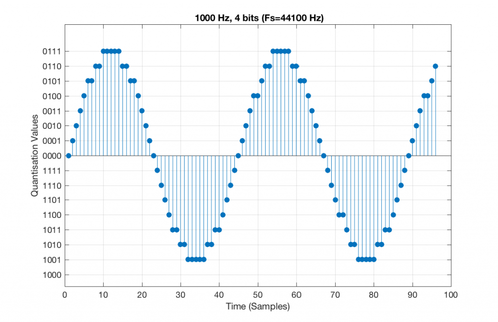
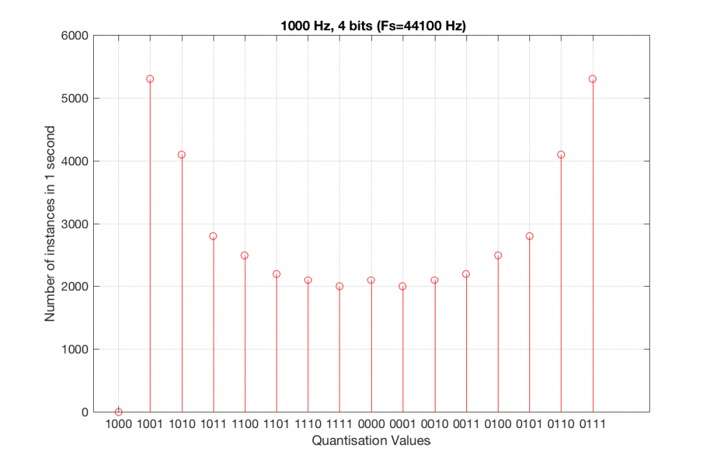
Compare Figures 6 and 8. Notice that Figure 8 appears to be a “smoother” shape. This is due to the fact that the instances of the waveform are not identical copies of each other. As can be seen in Figure 7, the waveform is slightly different. Of course, after a full second, then the whole cycle repeats itself, since there are 1000 cycles per second in the signal, and 44100 samples per second. If the signal were 1000.1 Hz, then it would take 10 seconds for the repetition to start.

Let’s increase the number of bits and see what happens. We’ll take it up to 6 bits.

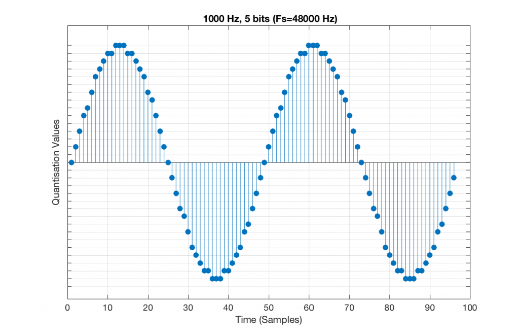
Figure 9 shows a 1 kHz sine tone in a 5-bit, 48 kHz system. Again, since 48000/1000 = 48, the two cycles are identical to each other. However, something new has happened here. If you look carefully at the positive side of the sine wave, you may notice that there are 5 quantisation values that are never used. On the negative side, there are 3 unused values, as well as the very bottom one.

So, because we are in a 5-bit system, we have 2^5 = 32 possible quantisation values, but, because we are using a 1 kHz sine tone, 9 of those possible values are never used. As a result, our histogram looks like Figure 10, below.

 

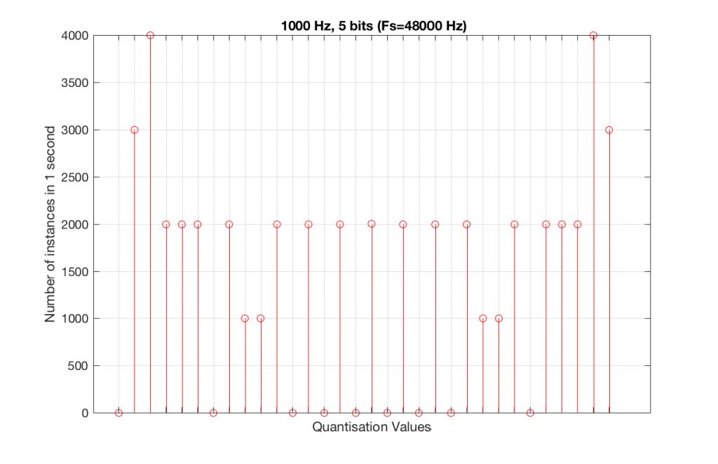
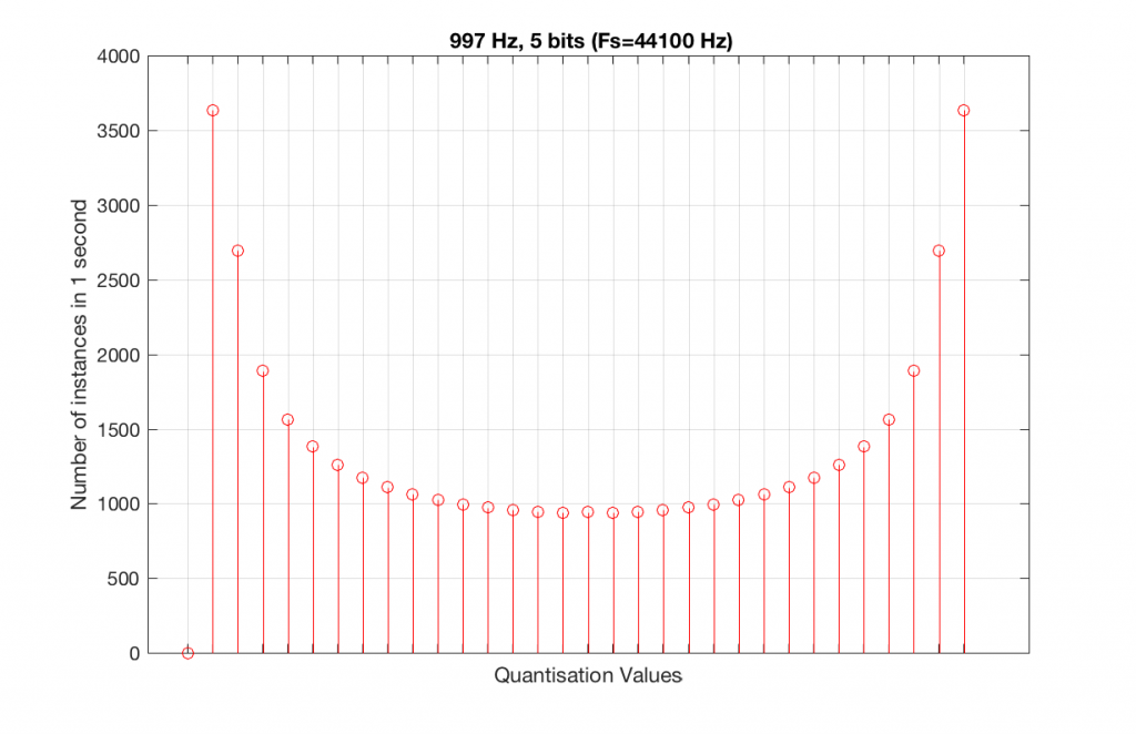
Let’s now compare that to a 5-bit, 44.1 kHz system.

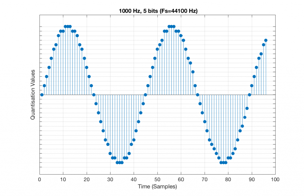
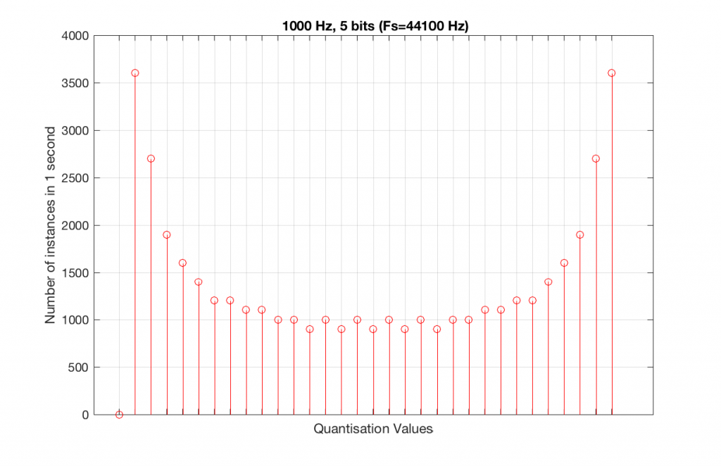
We can see that there is a basic problem here. The behaviour of the system may be different due only to the relationship between the sampling rate and the frequency of the signal.

The question is “what do we do about this?” We can see from Figures 10 and 12 that, when the signal’s frequency is not a nice round divisor of the sampling rate, we stand a better chance of testing the system more completely. So, instead of using a “nice” frequency like 1000 Hz, let’s use something close, but different enough to make things “misbehave” a little. One possible solution is to use 997 Hz, as we can see below:

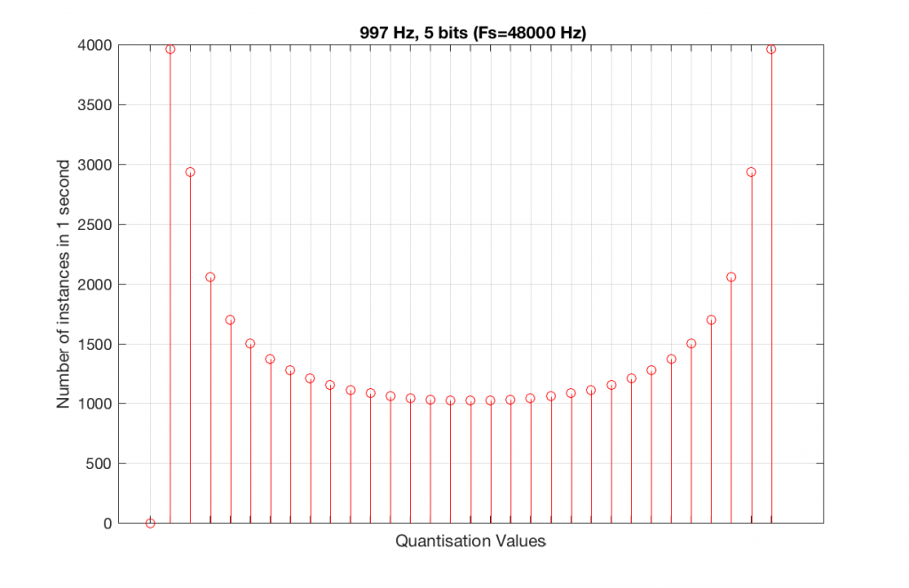
As can be seen in the histograms in Figure 13 and 14, changing the signal to 997 Hz from 1000 Hz results in us using all of the quantisation values in both sampling rates. So, we do a more thorough test, and stand a better chance of not missing anything…

 

At this point, you might say, “yes, but normally we used far more than 5 or 6 bits – this won’t happen in a system with more bits…” Nice try, but actually, things get worse, as you can see in Figures 15 and 16, below.

 

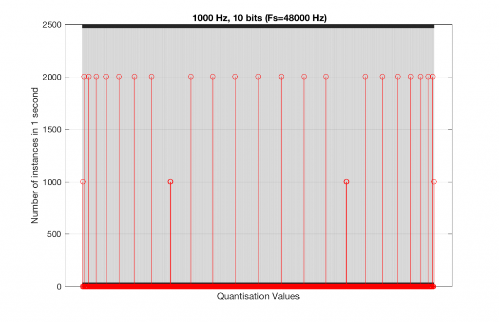
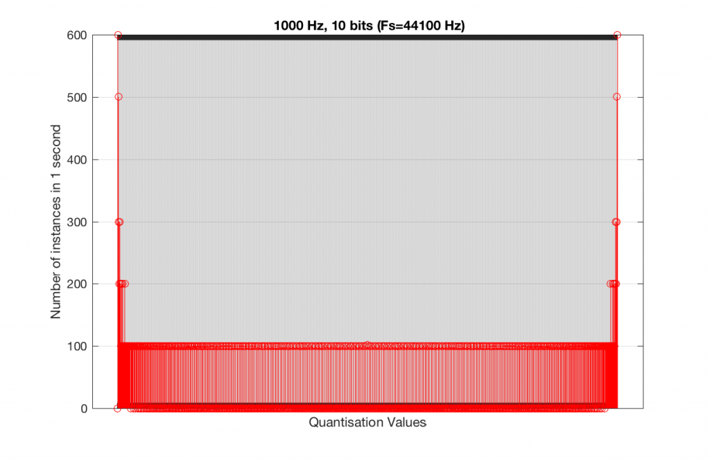
As you can see in Figures 15 and 16, lots of quantisation values are unused in both sampling rates with a 1 kHz signal. By comparison, if we used a 997 Hz tone, the results would be very different, as is shown in Figures 17 and 18.

 

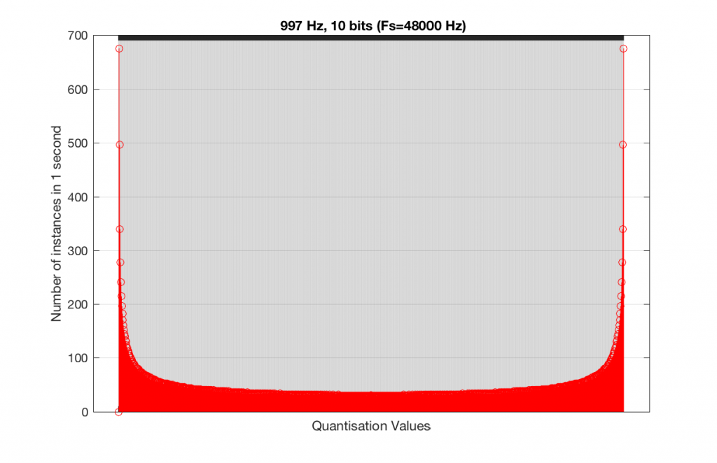
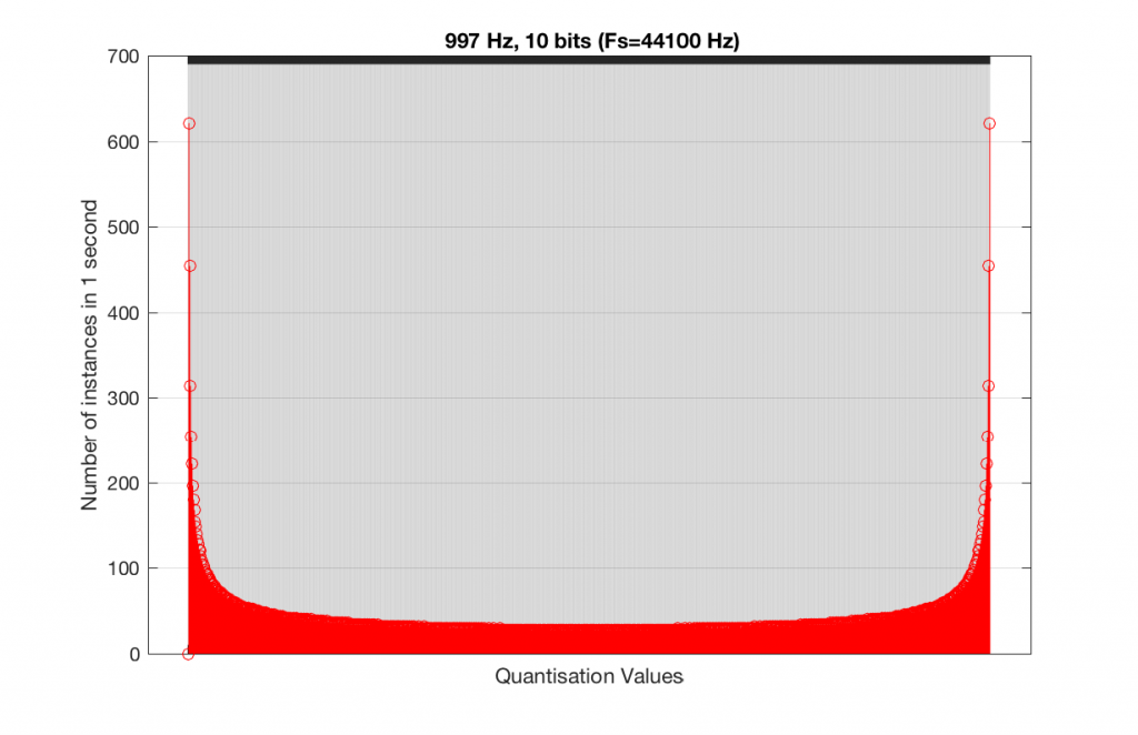
In fact, as we get more and more bits of resolution, the worse the problem gets, since we have an increasing number of available of quantisation values (increasing by a factor of 2 every time we add another bit), but the number of values that we use does not increase.

This is because, at some time, we start repeating the cycle. If the sampling rate divided by the signal frequency is an integer value (like a 1 kHz tone in a 48 kHz system), then we don’t use any new quantisation values after the first cycle of the tone (or 1 ms, in this case). If the sampling rate divided by the signal frequency is not an integer value (like a 997 Hz tone in a 48 kHz system) then we don’t start repeating ourselves until 1 second has passed.

However, think back to a comment that I made up at the top – if signal does start repeating itself after 1 second (in other words, if the frequency is an integer value), and if the number of samples per second is smaller than the number of quantisation values, then we will start repeating ourselves after 1 second, and we will only test the number of quantisation values that is equal to the sampling rate.

For example, if you have a 16-bit system, then you have 65536 possible quantisation values. If the sampling rate is 48000 Hz then we could only test a maximum of 48000 possible quantisation values out of the 65536 possible ones in one second, regardless of the frequency that we choose. Typically, however, we test fewer than this, because of the repetition of some values (e.g. the maximum value, if you have a periodic signal with a frequency greater than 1 Hz).

If we do this for the two frequencies we’ve been looking at – 1 kHz and 997 Hz, for two sampling rates, 44.1 kHz and 48 kHz, at different bit depths, the results look like the following figures.

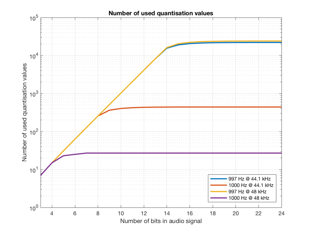
Notice in Figure 17 that the total number of quantisation values that are used when you have a 1 kHz tone in a 48 kHz system does not increase once you hit a word length of 7 bits. That does not mean that the signal’s representation does not improve – it does, since the quantisation values that you are using have a better resolution – so you’re rounding off less, so the error is smaller.

Notice as well that the 997 Hz tone not only results in us using far more quantisation values (topping out at the sampling rates) than the 1000 Hz tone, but that they are more similar in the two sampling rates.

If we plot the number of unused samples instead, it looks like Figure 18.

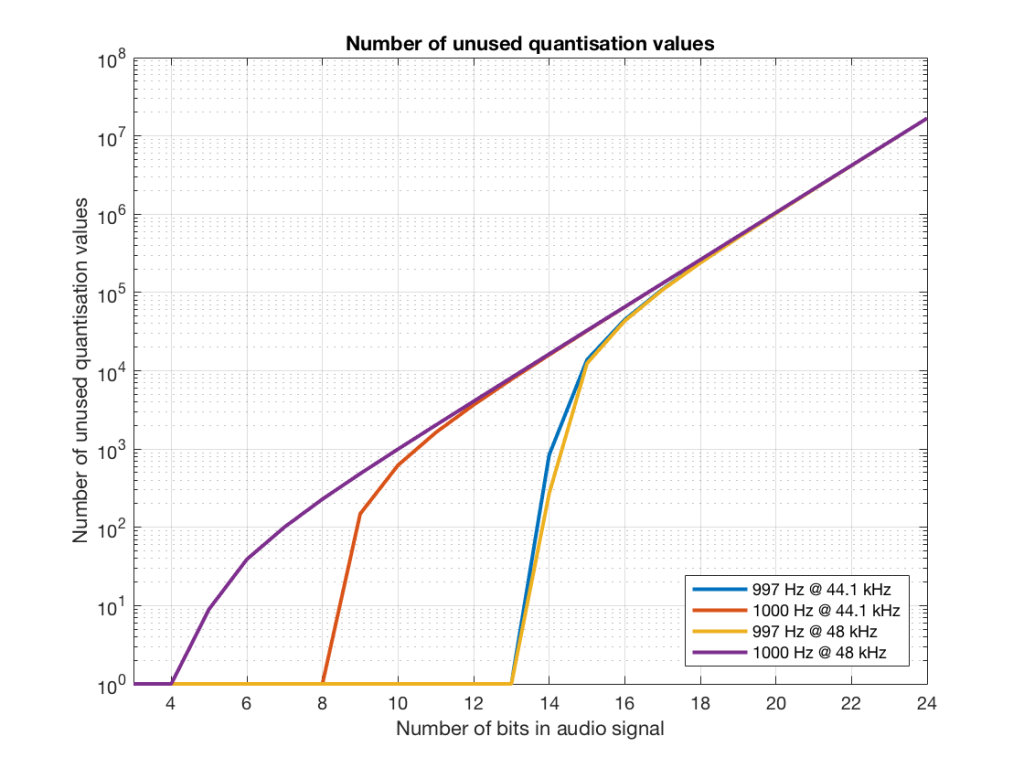
Figure 18 is a little misleading, since as the bit depth increases, the total possible number of quantisation values also increases, however, since the two frequencies that we are analysing are integer values, the maximum number cannot go past the sampling rate. So, in an extreme case (if you choose your frequency or signal carefully), only 48000 values out of a possible 16777216 values are used in a 24-bit system per second in a system with a sampling rate of 48 kHz.

Figure 19 shows the same information as Figure 18, except that I’ve displayed the values in percent.

 

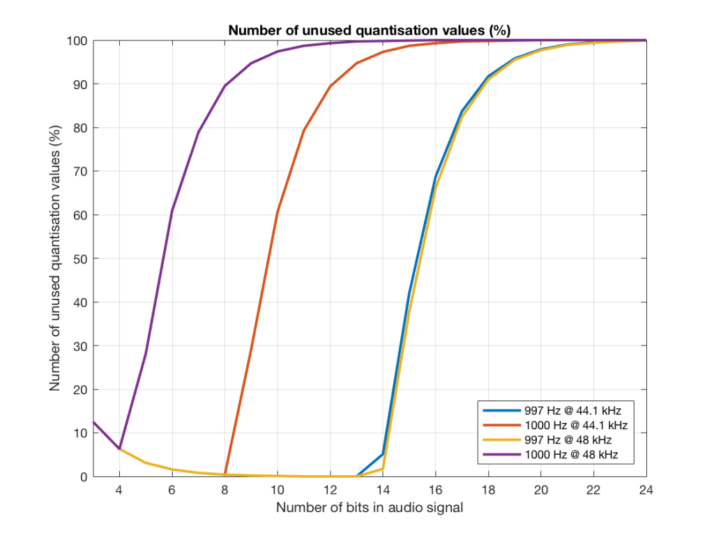
So, as you can see there, in a 16-bit system, even if you use a 997 Hz tone, about 70% of the total possible quantisation values are used.

 

Caveat

Of course, the signals that I used here were generated digitally, and did not include dither. If I had included proper dithering, then more of the quantisation values would have been used. However, the point of this posting was not to talk about correct ways of creating PCM signals – it was an attempt to explain why we use 997 Hz instead of 1 kHz when we test digital audio systems.