Last week, I was doing a lecture about the basics of audio and I happened to mention one of the rules of thumb that we use in loudspeaker development:

If you have a single loudspeaker driver and you want to keep the same Sound Pressure Level (or output level) as you change the frequency, then if you go down one octave, you need to increase the excursion of the driver 4 times.

One of the people attending the presentation asked “why?” which is a really good question, and as I was answering it, I realised that it could be that many people don’t know this.

Let’s take this step-by-step and keep things simple. We’ll assume for this posting that a loudspeaker driver is a circular piston that moves in and out of a sealed cabinet. It is perfectly flat, and we’ll pretend that it really acts like a piston (so there’s no rubber or foam surround that’s stretching back and forth to make us argue about changes in the diameter of the circle). Also, we’ll assume that the face of the loudspeaker cabinet is infinite to get rid of diffraction. Finally, we’ll say that the space in front of the driver is infinite and has no reflective surfaces in it, so the waveform just radiates from the front of the driver outwards forever. Simple!

Then, we’ll push and pull the loudspeaker driver in and out using electrical current from a power amplifier that is connected to a sine wave generator. So, the driver moves in and out of the “box” with a sinusoidal motion. This can be graphed like this:

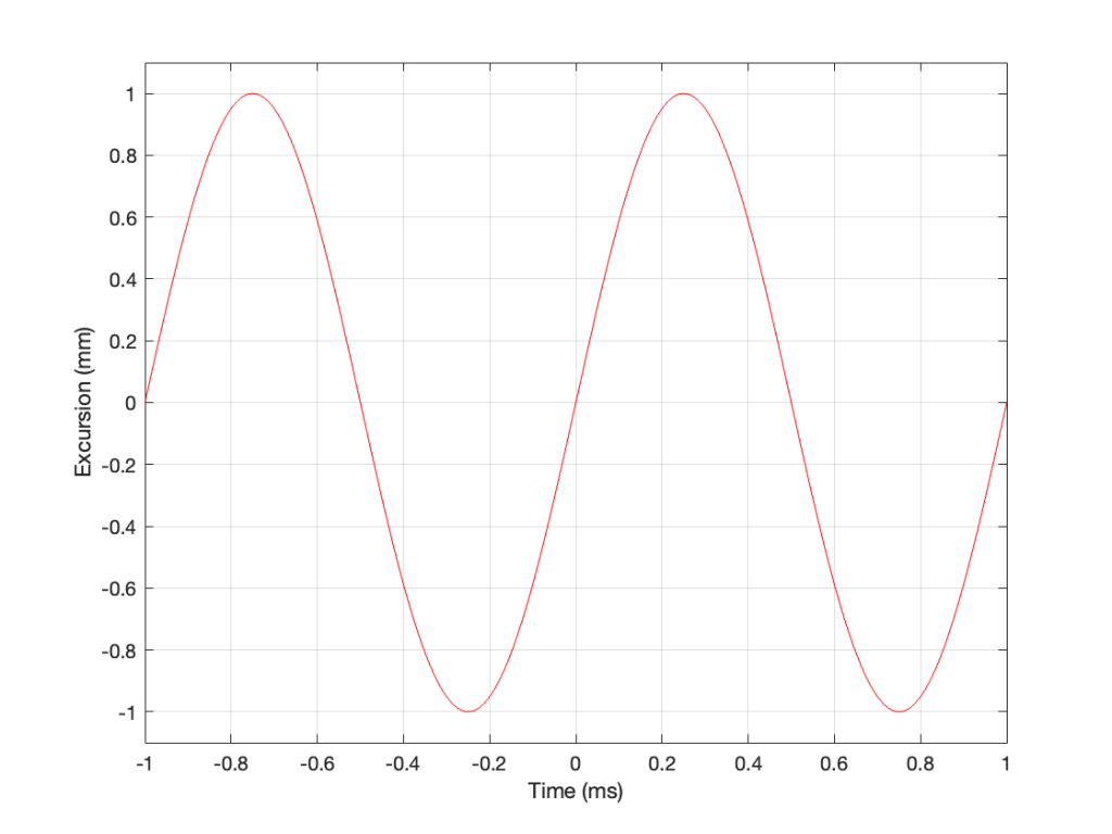
As you can see there, we have one cycle per millisecond, therefore 1000 cycles per second (or 1 kHz), and the driver has a peak excursion of 1 mm. It moves to a maximum of 1 mm out of the box, and 1 mm into the box.

Consider the wave at Time = 0. The driver is passing the 0 mm line, going as fast as it can moving outwards until it gets to 1 mm (at Time = 0.25 ms) by which time it has slowed down and stopped, and then starts moving back in towards the box.

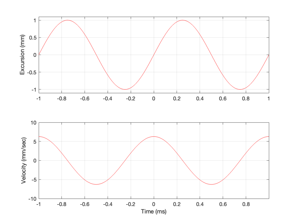
So, the velocity of the driver is the slope of the line in Figure 1, as shown in Figure 2.

As the loudspeaker driver moves in and out of the box, it’s pushing and pulling the air molecules in front of it. Since we’ve over-simplified our system, we can think of the air molecules that are getting pushed and pulled as the cylinder of air that is outlined by the face of the moving piston. In other words, its a “can” of air with the same diameter as the loudspeaker driver, and the same height as the peak-to-peak excursion of the driver (in this case, 2 mm, since it moves 1 mm inwards and 1 mm outwards).

However, sound pressure (which is how loud sounds are) is a measurement of how much the air molecules are compressed and decompressed by the movement of the driver. This is proportional to the acceleration of the driver (neither the velocity nor the excursion, directly…). Luckily, however, we can calculate the driver’s acceleration from the velocity curve. If you look at the bottom plot in Figure 2, you can see that, leading up to Time = 0, the velocity has increased to a maximum (so the acceleration was positive). At Time = 0, the velocity is starting to drop (because the excursion is on its was up to where it will stop at maximum excursion at time = 0.25 ms).

In other words, the acceleration is the slope of the velocity curve, the line in the bottom plot in Figure 2. If we plot this, it looks like Figure 3.

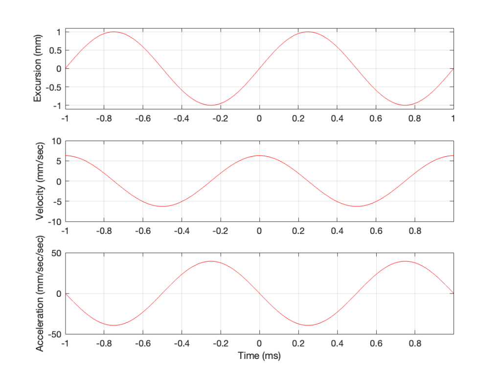
Now we have something useful. Since the bottom plot in Figure 3 shows us the acceleration of the driver, then it can be used to compare to a different frequency. For example, if we get the same driver to play a signal that has half of the frequency, and the same excursion, what happens?

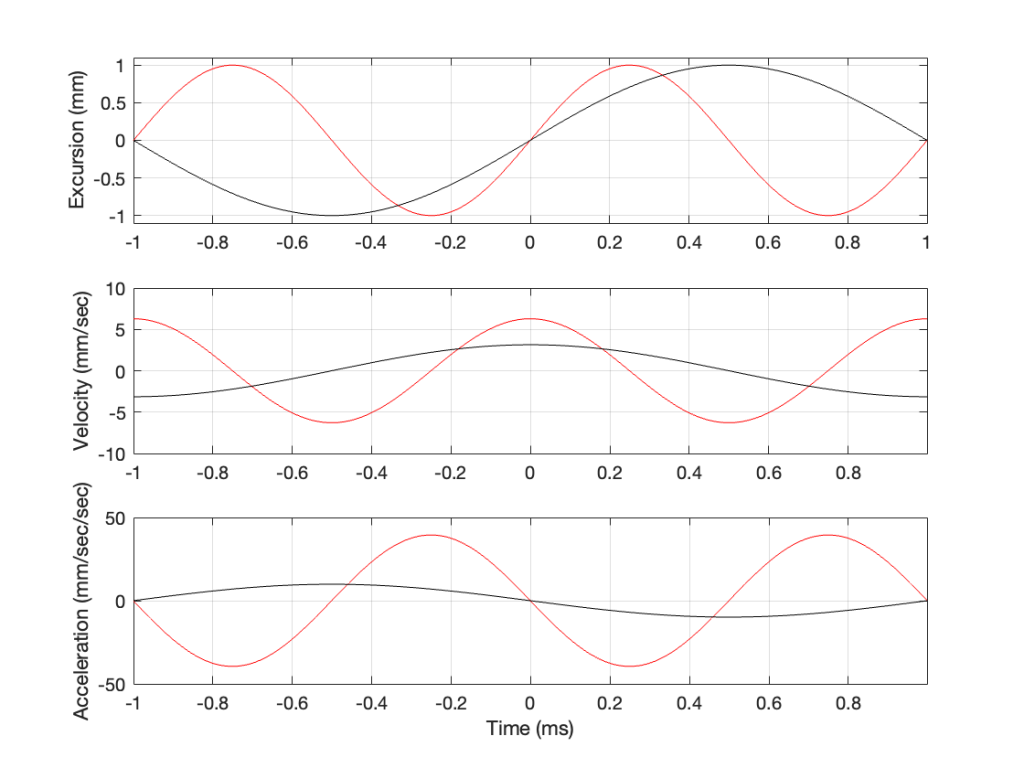
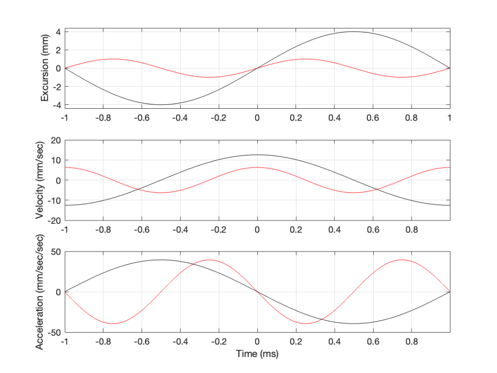
In Figure 4, two sine waves are shown: the black line is 1/2 of the frequency of the red line, but they both have the same excursion. If you take a look at where both lines cross the Time = 0 point, then you can see that the slopes are different: the red line is steeper than the black. This is why the peak of the red line in the velocity curve is higher, since this is the same thing. Since the maximum slope of the red line in the middle plot is higher than the maximum slope of the black line, then its acceleration must be higher, which is what we see in the bottom plot.

Since the sound pressure level is proportional to the acceleration of the driver, then we can see in the top and bottom plots in Figure 4 that, if we halve the frequency (go down one octave) but maintain the same excursion, then the acceleration drops to 25% of the previous amount, and therefore, so does the sound pressure level (20*log10(0.25) = -12 dB, which is another way to express the drop in level…)

This raises the question: “how much do we have to increase the excursion to maintain the acceleration (and therefore the sound pressure level)?” The answer is in the “25%” in the previous paragraph. Since maintaining the same excursion and multiplying the frequency by 0.5 resulted in multiplying the acceleration by 0.25, we’ll have to increase the excursion by 4 to maintain the same acceleration.

Looking at Figure 5: The black line is 1/2 the frequency of the red line. Their accelerations (the bottom plots) have the same peak values (which means that they produce the same sound pressure level). This, means that the slopes of their velocities are the same at their maxima, which, in turn, means that the peak velocity of the black line (the lower frequency) is higher. Since the peak velocity of the black line is higher (by a factor of 2) then the slope of the excursion plot is also twice as steep, which means that the peak of the excursion of the black line is 4x that of the red line. All of that is explained again in Figure 6.

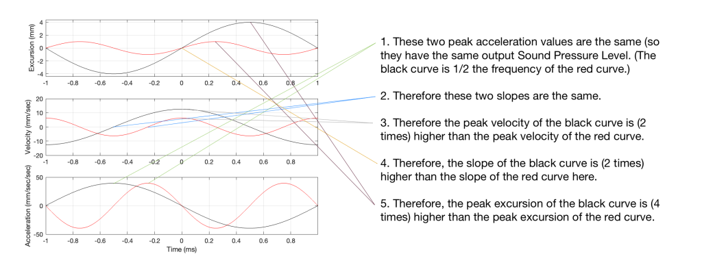
Therefore, assuming that we’re using the same loudspeaker driver, we have to increase the excursion by a factor of 4 when we drop the frequency by a factor of 2, in order to maintain a constant sound pressure level.

However, we can play a little trick… what we’re really doing here is increasing the volume of our “cylinder” of air by a factor of 4. Since we don’t change the size of the driver, we have to move it 4 times farther.

However, the volume of a cylinder is

π r² * height

and we’re just playing with the “height” in that equation. A different way would be to use a different driver with a bigger surface area to play the lower frequency. For example, if we multiply the radius of the driver by 2, and we don’t change the excursion (the “height” of the cylinder) then the total volume increases by a factor of 4 (because the radius is squared in the equation, and 2*2 = 4).

Another way to think of this: if our loudspeaker driver was a square instead of a circle, we could either move it in and out 4 times farther OR we would make the width and the length of the square each twice as big to get the a cube with the same volume. That “r²” in the equation above is basically just the “width * length” of a circle…

This is why woofers are bigger than tweeters. In a hypothetical world, a tweeter can play the same low frequencies as a woofer – but it would have to move REALLY far in and out to do it.