Every once-in-a-while, I have to measure a system to find out whether its clock is behaving, or at the very least, whether its latency is stable over time. There are a number of different ways to do this, but I was trying to find a way that would be quick to implement and simple to analyse, if only as an initial “smoke test” to determine whether the system is working perfectly (which never happens) or which measurements we have to do next in order to figure out what exactly is going on.
Anyone who works in an engineering-type of area knows that the job doesn’t stop when you go home for the day. It percolates in the back of your head until, while you’re distracted by something else, the answer you’ve been looking for bubbles up to the frontal lobe. So, one evening I’m walking the dog in the forest, in the rain, and, like most people do, I was thinking about why we use 997 Hz sine tones to measure digital audio systems (if you don’t know the answer to this, check this posting). And that’s where it hit me. If we use a weird number to try and hit as many quantisation values as possible, what happens if we do the opposite?
Here’s a plot of a 4800 Hz sine tone, sampled at 48 kHz.
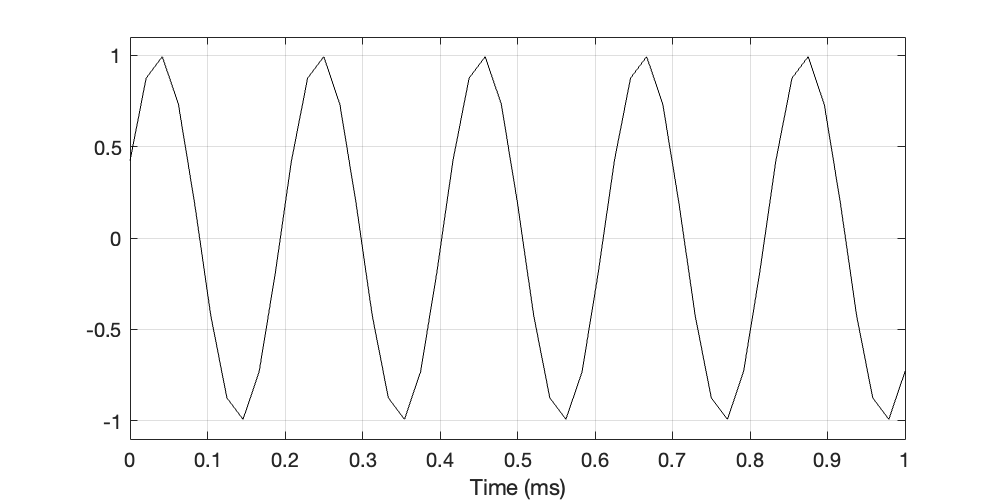
This is the way we normally plot a digital audio signal, but it’s not really fair. What I’m doing there is to connect the sample values. However, when this signal is sent out of a DAC, it will be smoothed by a reconstruction filter so those sharp corners will disappear on their way out to the real world. However, for the purposes of this posting, this doesn’t matter, since what I’m really interested in are the sample values themselves, as shown in Figure 2.
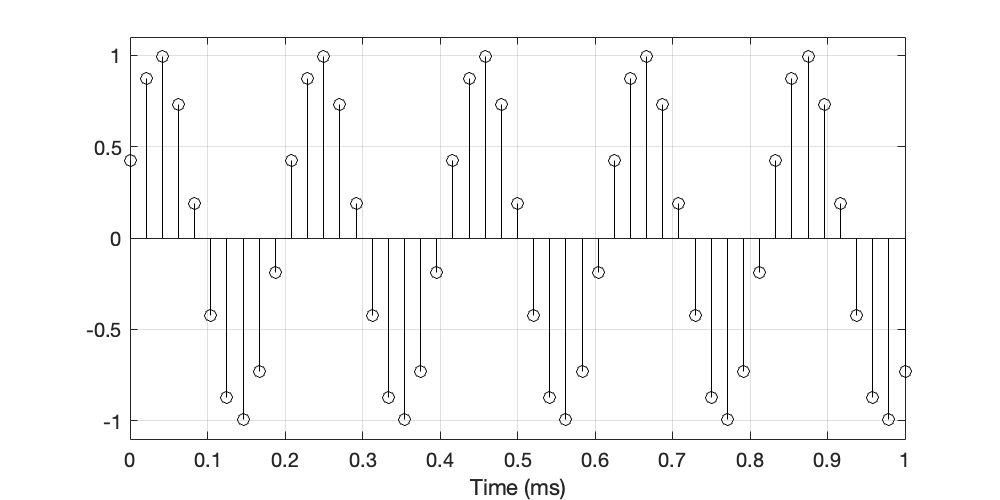
You may notice something curious about this plot. Since I’ve chosen to plot a sine wave whose frequency is exactly 1/10th of the sampling rate, then each period of the waveform is 10 samples long, and the next period is identical to the previous one. This can be shown by connecting every 10th sample as shown in Figure 3.

Again a reminder: this is the reason we use the “weird” frequency of 997 Hz to test a digital audio system running at 44.1 kHz or 48 kHz.
In this case, testing a 48 kHz system with a 4.8 kHz tone can measure 10 sample values at most. (If I had chosen to start with a different phase, it might have been fewer sample values, since I would have gotten repetitions within a period.)
If I “connect the dots” for all 10 sample values, it will look like Figure 4.
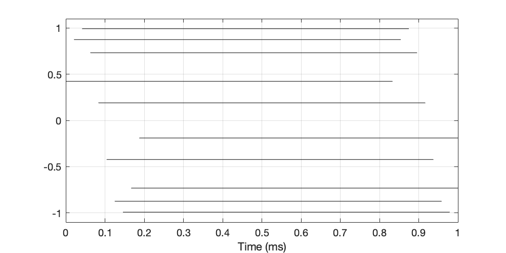
If I then do that for a much longer time window, it will look basically the same; I just won’t be able to see when the lines start and stop because we’ve zoomed out.

What will happen to this plot if the clock is drifting? For example, if you’re playing a 4.8 kHz tone through a system that is NOT running at 48 kHz (even though it should), then the samples won’t appear at the right time, and so they will have a different instantaneous amplitude. In other words, a change in time will result in a change in phase, which will show up in a plot like the one in Figure 5 as a change in amplitude.
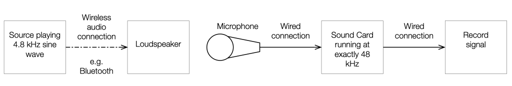
Let’s pretend that we set up a system like the one shown above, and let’s say that the signal that we record over there on the right hand side produces a plot like the one shown below in Figure 7.

What does Figure 7 show us? Since the recording that we made with the sound card is at exactly 48 kHz, and since these are not horizontal lines, then this means that the recorded signal is not exactly 4.8 kHz.
However, this does not necessarily mean that the source (on the left side of Figure 6) is not transmitting a 4.8 kHz sine tone. It could mean that the clock that is determining the sampling rate in the loudspeaker is incorrect. So, the source “thinks” it’s playing a 4.8 kHz tone, but the loudspeaker is deciding otherwise for some reason. (This is a very normal behaviour. Nothing is perfect, and a Bluetooth speaker is a likely suspect for a number of errors…)
The curves in Figure 7 are sinusoidal. This means that the drift is constant. In other words, the sampling rate is wrong, but not varying, resulting in the wrong frequency of sine wave being played – but at least the frequency is not modulating. We can also see that each of the 10 sinusoidal waves makes about 1 cycle in the 1000 ms of the plot. This means that the clock is drifting by 1 period of the audio sine wave (4.8 kHz) ever 1000 ms. In other words, this is a system that it actually running at either 47990 Hz or 48010 Hz instead of 48000 Hz (because we’re either gaining or losing 10 samples every second). Unfortunately, without a little more attention, we don’t even know whether we’re running too slowly or too fast…
If the playback system’s clock (which controls its sampling rate) is not just incorrect but unstable, then you might see something like Figure 8, where I’ve only connected one of the 10 samples values.
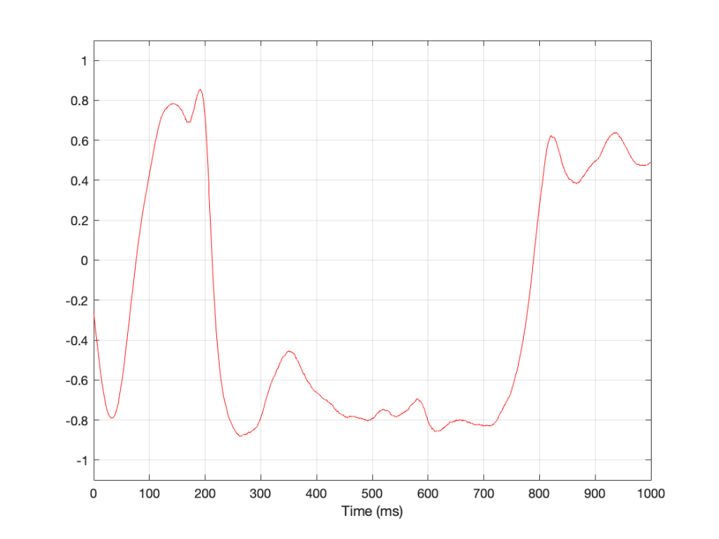
If I were to plot the same slice of time, showing all 10 samples in the sine wave, they would look like Figure 9. Admittedly, this is probably less useful than Figure 8.
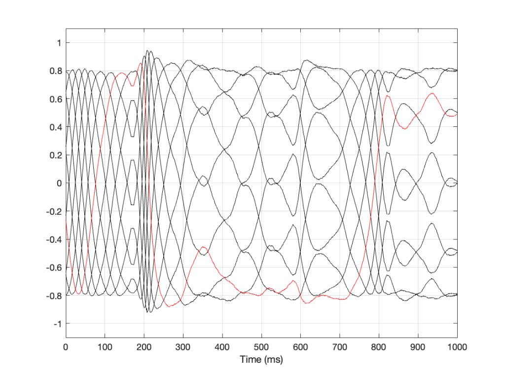
Obviously, this doesn’t tell us what’s going on other than to say that it’s obvious that this system is NOT behaving. However, we can get a little useful information. For example, we can see that the clock drift is modulating more from 0 ms to 200 ms, and then settles down to a more stable (and more correct) value from 200 to about 600 ms.
It would take more analysis to learn enough about this system to know what’s happening. However, as a smoke test to let you know whether it’s behaving well enough to not worry too much, or to see where you need to “zoom in” to find out more information.