
If you’re interested in underwater bioacoustics, naval warfare, or crustacea, this podcast is for you!
If you’re interested in underwater bioacoustics, naval warfare, or crustacea, this podcast is for you!
#52 in a series of articles about the technology behind Bang & Olufsen loudspeakers
I often have to do demos of loudspeakers for people. Also, I frequently have to make recommendations on how to do (either for Bang & Olufsen dealers, or for things like press events). One of the problems that I face every time I have to do this is how to arrange the chairs so that everyone gets a reasonable impression of how a loudspeaker sounds. The problem is that this is basically impossible, due to the significant influence things like the loudspeakers’ locations, the listener location, and the room, have on the overall sound.
One aspect of how-a-loudspeaker-sounds is its magnitude response (often called a “frequency response”). A (perhaps too-simple) definition of a magnitude response is “a measure of how loud the output signal is at different frequencies if you put in a signal that is the same level at all frequencies”.
If we wanted to make a measurement of a loudspeaker’s magnitude response in a room at a particular position, we just have to put in a signal that contains all frequencies at the same magnitude (or level), capture that output with a microphone somewhere in the room, and compare how loud the signal is at different frequencies. Of course, in order to do this, we have to take care of some details. We have to make sure that the microphone (and everything else in the measurement part of the signal path) has a flat magnitude response. If it doesn’t, then at least we should know what its response is, so we can subtract it from the measurement to remove its influence on the result.
However, for the purposes of this posting, I’m not really interested in the absolute response of a loudspeaker. I’m more interested in how that response changes as you move in a room. Specifically, I want to show how much the magnitude response can change with very small changes in listening position.
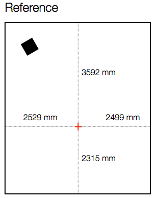
Let’s start by measuring the magnitude response of a loudspeaker in a room at a location. For the purposes of this example, I’ve used a full-range, multi-way loudspeaker without a port. It’s placed roughly 1 m from the side wall and 1 m from the front wall, aimed at a listening position. The listening position is in the centre of the room’s width, and closer to the rear wall than the front wall by about a metre. The details of the location for the microphone (a 1/4″ omnidirectional measurement mic) for this measurement are shown in Figure 1, below.
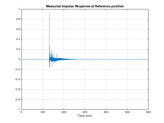
I did an impulse response measurement (using an MLS signal with 4 averages (to improve SNR) and 4 sequences (to reduce the effect of distortion)) of the loudspeaker, the result of which is shown below in Figure 2. As you can see there, there are many obvious reflections after the initial impulse, and there is some kind of ringing in the room’s response.
The extremely long time before the onset of the impulse is arbitrary. The microphone was not actually 40 m away from the loudspeaker…
As I said above, I’m not interested in the resulting magnitude response of this measurement. I can tell you that it’s messy. There are bumps and dips in the low end caused (primarily) by room modes. The top end is messy due to the reflections. The overall curve is not flat due to the loudspeaker’s response, the microphone’s orientation, and various components in the signal path. However, I don’t care, since I’m not here to measure how the speaker behaves at one location in the room. I’m here to find out how its behaviour changes when you change location. So, let’s move the microphone.
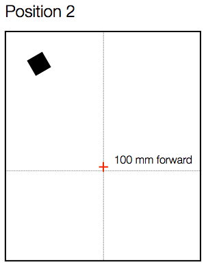
As you can see in Figure 3, below, I started by moving the microphone only 100 mm, directly forwards in the room.
Again, I measured the impulse response, converted that to a magnitude response (reflections and all!), smoothed it with a running 1/3 octave smoothing and subtracted the magnitude response measured at the Reference position (also smoothed to 1/3 octave). The resulting difference is shown in Figure 4, below.
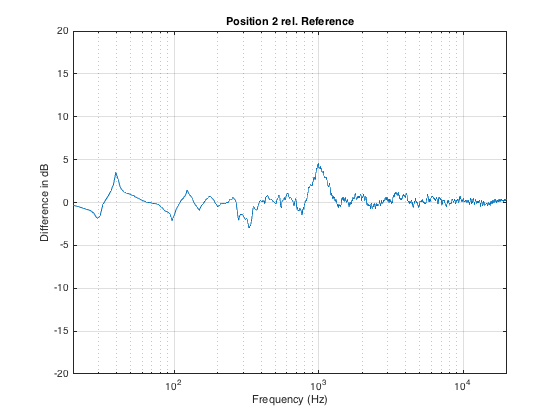
As you can see in Figure 3, moving the listening position only 100 mm results in a magnitude response deviation of about -2 to +4 dB. This is easily within the threshold of audibility for most people…
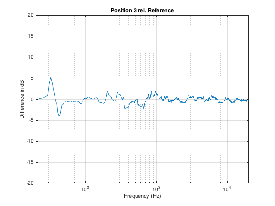
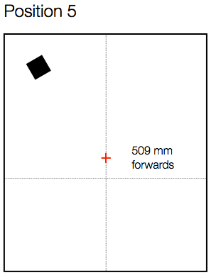
Now, let’s move the microphone sideways instead, as shown in Figure 5.
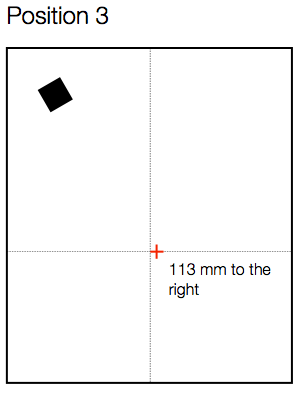
Again, a roughly 100 mm movement results in a large change in the magnitude response – although now the most significant changes have happened in the low end, as can be seen in Figure 6.
If we have more than one listener attending the demo, then I prefer to seat them “bus” style – one directly in front of the other – to ensure that everyone is getting a reasonably good phantom centre image. Sitting off-centre results in the time of arrival of signals from the two loudspeakers being mis-matched which will result in phantom images pulling towards the closer (and therefore earlier) loudspeaker.
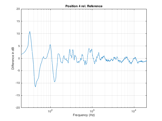
Let’s say the we have a person roughly a half-metre behind the “good” chair, as shown in Figure 7. How different is the sound in that location?
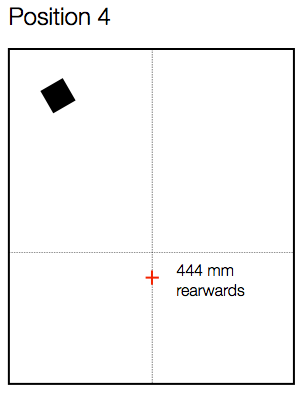
Now we can see in Figure 8 that, by moving backwards in the room, we get more than ± 10 dB of variation in the magnitude response, with significant deviations happening as high as 1 kHz (depending on how you define “significant”).
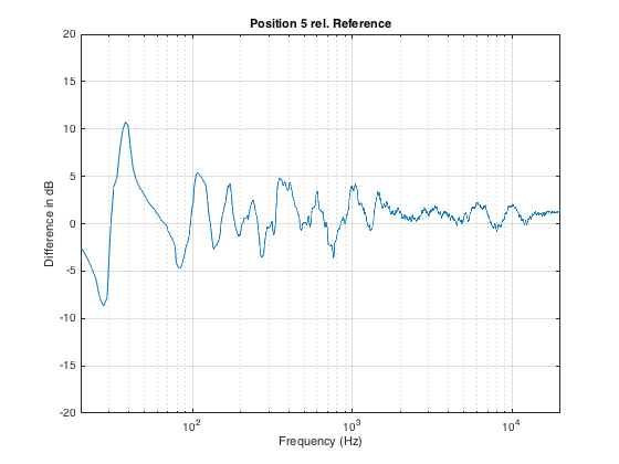
Similarly, moving forwards by a half metre from the Reference position (shown in Figure 9) results in a similar amount of change in the magnitude response, shown in Figure 10.
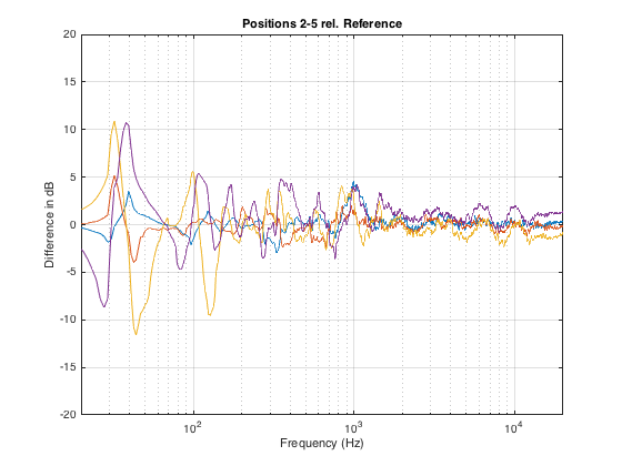
Just for comparison, I’ve re-plotted the 4 magnitude response differences shown above in one plot. This is to show that the changes are not necessarily easily predicable with a simple knowledge of room layout. In other words, it would be almost impossible, without some serious simulation software, to predict these changes just by looking at a floorplan of the room and the chairs.
What’s the moral of the story here? There are many – but I’ll just mention three.
The first is the message that, even a very small change in location (like leaning to one side in your chair – or leaning forwards to rest your elbows on your knees and your chin on your hands) can dramatically change the simple magnitude response of a loudspeaker (we won’t get into the effects on the spatial behaviour of the system).
The second is that, when you’re sitting with a friend, auditioning a pair of loudspeakers, switch chairs now and again. It is extremely unlikely that you’re both hearing the same thing at the same time.
Thirdly, the fact that there are significant differences between magnitude responses at different listening positions (even within a half-metre radius) means that, if you’re doing measurements for a room compensation system using a microphone around the listening position, it’s always smarter to make more than one measurement. In fact, there are some people who argue that, in this case, having only one measurement is worse than having no measurements, since you can easily get distracted by something in the magnitude or the time response that is a problem at only that location and nowhere else.
Finally, it’s worth considering that first point a different way. Let’s say you’re the type of person who likes to tweak a stereo system by upgrading components like wires. And, let’s say that you have incredible powers of “sonic memory” – in other words, you can listen to a system, take a break, listen to it again, and you are able to detect extremely small changes in system performance (like the magnitude response). So, you listen to your system – then you get out of your chair, change the component, sit down again, and start listening to the same tune at the same level. Remember that, unless you are in exactly the same location that you were before (not just “in the same chair”…), it could be that there is a larger difference in the magnitude response of the loudspeaker due your change in position than there is due to the component you just changed… So if you are a tweaker – get someone else to do the dirty work for you so you can sit there, in your chair, with your head in a clamp, waiting to evaluate the “upgrade”…
“Everybody knows” that noise-induced hearing loss is a problem for rock musicians. This has been reported by standard media like in this article and this press release from AC/DC, and in more “scientific” journals like in this article. However, what seems to be less-widely considered is that classical musicians have exactly the same problems…


#51 in a series of articles about the technology behind Bang & Olufsen loudspeakers
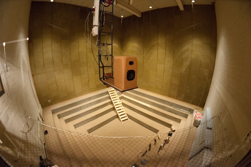
Sometimes, we have journalists visiting Bang & Olufsen in Struer to see our facilities. Of course, any visit to Struer means a visit to The Cube – our room where we do almost all of the measurements of the acoustical behaviour of our loudspeaker prototypes. Different people ask different questions about that room – but there are two that come up again and again:
Of course, the level of detail of the answer is different for different groups of people (technical journalists from audio magazines get a different level of answer than lifestyle journalists from interior design magazines). In this article, I’ll give an even more thorough answer than the one the geeks get. :-)
Our goal, when we measure a loudspeaker, is to find out something about its behaviour in the absence of a room. If we measured the loudspeaker in a “real” room, the measurement would be “infected” by the characteristics of the room itself. Since everyone’s room is different, we need to remove that part of the equation and try to measure how the loudspeaker would behave without any walls, ceiling or floor to disturb it.
So, this means (conceptually, at least) that we want to measure the loudspeaker when it’s floating in space.
Basically, the measurements that we perform on a loudspeaker can be boiled down into four types:
Luckily, if you’re just a wee bit clever (and we think that we are…), all four of these measurements can be done using the same basic underlying technique.
The very basic idea of doing any audio measurement is that you have some thing whose characteristics you’re trying to measure – the problem is that this thing is usually a link in a chain of things – but you’re only really interested in that one link. In our case, the things in the audio chain are electrical (like the DAC, microphone preamplifier, and ADC) and acoustical (like the measurement microphone and the room itself).
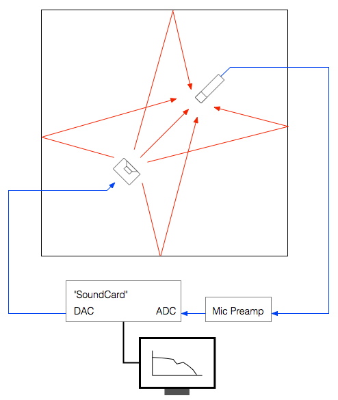
The computer sends a special signal (we’ll come back to that…) out of its “sound card” to the input of the loudspeaker. The sound comes out of the loudspeaker and comes into the microphone (however, so do all the reflections from the walls, ceiling and floor of the Cube). The output of the microphone gets amplified by a preamplifier and sent back into the computer. The computer then “looks at” the difference between the signal that it sent out and the signal that came back in. Since we already know the characteristics of the sound card, the microphone and the mic preamp, then the only thing remaining that caused the output and input signals to be different is the loudspeaker.
There are lots of different ways to measure an audio device. One particularly useful way is to analyse how it behaves when you send it a signal called an “impulse” – a click. The nice thing about a theoretically perfect click is that it contains all frequencies at the same amplitude and with a known phase relationship. If you send the impulse through a device that has an “imperfect” frequency response, then the click changes its shape. By doing some analysis using some 200-year old mathematical tricks (called “Fourier analysis“), we can convert the shape of the impulse into a plot of the magnitude and phase responses of the device.
So, we measure the way the device (in our case, a loudspeaker) responds to an impulse – in other words, its “impulse response”.
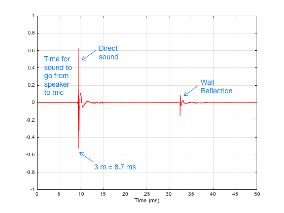
There are three things to initially notice in this figure.
In order to get a measurement of the loudspeaker in the absence of a room, we have to get rid of those reflections… In this case, all we have to do is to tell the computer to “stop listening” before that reflection arrives. The result is the impulse response of the loudspeaker in the absence of any reflections – which is exactly what we want.
Great. That’s a list of the basic measurements that come out of The Cube. However, I still have’t directly answered the original questions…
Let’s take the second question first: “Why isn’t The Cube an anechoic chamber?”
This raises the question: “What’s an anechoic chamber?” An anechoic chamber is a room whose walls are designed to be absorptive (typically to sound waves, although there are some chambers that are designed to absorb radio waves – these are for testing antennae instead of loudspeakers). If the walls are perfectly absorptive, then there are no reflections, and the loudspeaker behaves as if there are no walls.
So, this question has already been answered – albeit indirectly. We do an impulse response measurement of the loudspeaker, which is converted to magnitude and phase response measurements. As we saw in Figure 5, the reflections off the walls are easily visible in the impulse response. Since, after the impulse response measurement is done, we can “delete” the reflection (using a process called “windowing”) we end up with an impulse response that has no reflections. This is why we typically say that The Cube is “pseudo-anechoic” – the room is not anechoic, but we can modify the measurements after they’re done to be the same as if it were.
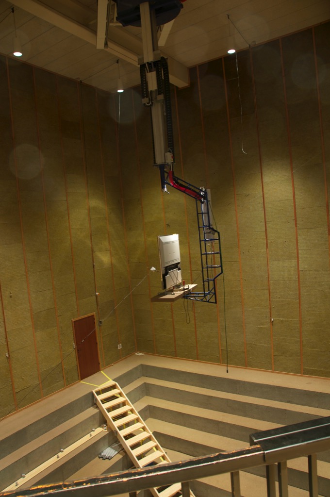
Now to the harder question to answer: “Why is the room so big?”
Let’s say that you have a device (for example, a loudspeaker), and it’s your job to measure its magnitude response. One typical way to do this is to measure its impulse response and to do a DFT (or FFT) on that to arrive at a magnitude response.
Let’s also say that you didn’t do your impulse response measurement in a REAL free field (a space where there are no reflections – the wave is free to keep going forever without hitting anything) – but, instead, that you did your measurement in a real space where there are some reflections. “No problem,” you say “I’ll just window out the reflections” (translation: “I’ll just cut the length of the impulse response so that I slice off the end before the first reflection shows up.”)
This is a common method of making a “pseudo-anechoic” measurement of a loudspeaker. You do the measurement in a space, and then slice off the end of the impulse response before you do an FFT to get a magnitude response.
Generally speaking, this procedure works fairly well… One thing that you have to worry about is a well-known relationship between the length of the impulse response (after you’ve sliced it) and the reliability of your measurement. The shorter the impulse response, the less you can trust the low-frequency result from your FFT. One reason for this is that, when you do an FFT, it uses a “slice” of time to convert the signal into a frequency response. In order to be able to measure a given frequency accurately, the FFT math needs at least one full cycle within the slice of time. Take a look at Figure 6, below.
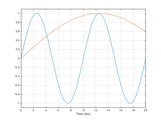
As you can see in that plot, if the slice of time that we’re looking at is 20 ms long, there is enough time to “see” two complete cycles of a 100 Hz sine tone (in blue). However, 20 ms is not long enough to see even one half of a cycle of a 20 Hz sine tone (in red).
However, there is something else to worry about – a less-well-known relationship between the level and extension of the low-frequency content of the device under test and the impulse response length. (Actually, these two issues are basically the same thing – we’re just playing with how low is “low”…)
Let’s start be inventing a loudspeaker that has a perfectly flat on-axis magnitude response but a low-frequency limitation with a roll-off at 10 Hz. I’ve simulated this very unrealistic loudspeaker by building a signal processing flow as shown in Figure 7.

If we were to do an impulse response measurement of that system, it would look like the plot in Figure 8, below.
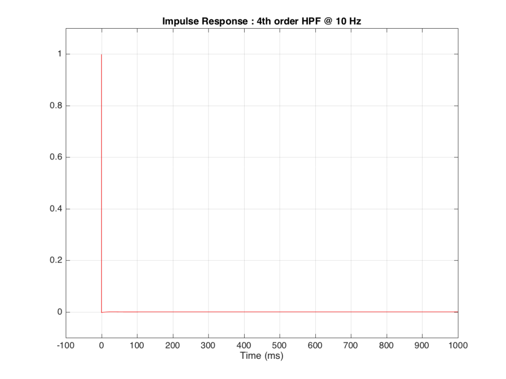
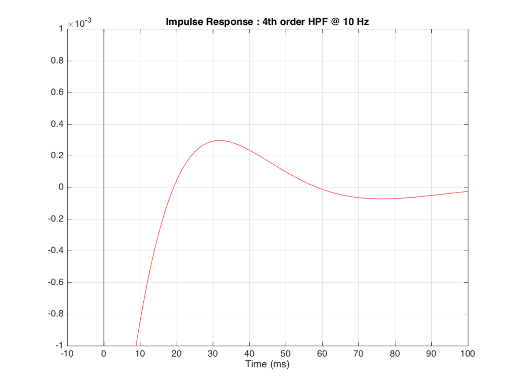
Figure 9, above shows a closeup of what happens just after the impulse. Notice that the signal drops below 0, then swings back up, then negative again. In fact, this keeps happening – the signal goes positive, negative, positive, negative – theoretically for an infinite amount of time – it never stops. (This is why the filters that I used to make this high pass are called “IIR” filters or “Infinite Impulse Response” filters.)
The problem is that this “ringing” in time (to infinity) is very small. However, it’s more easily visible if we plot it on a logarithmic scale, as shown below in Figure 10.
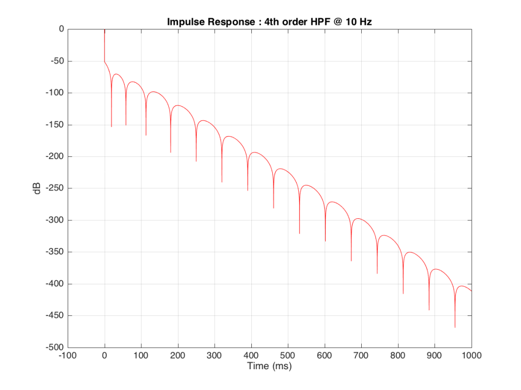
As you can see there, after 1 second (1000 ms) the oscillation caused by the filtering has dropped by about 400 dB relative to the initial impulse (that means it has a level of about 0.000 000 000 000 000 000 01 if the initial impulse has a value of 1). This is very small – but it exists. This means that, if we “cut off” the impulse to measure its frequency response, we’ll be cutting off some of the signal (the oscillation) and therefore getting some error in the conversion to frequency. The question then is: how much error is generated when we shorten the impulse length?
We won’t do an analysis of how to answer this question – I’ll just give some examples. Let’s take the total impulse response shown in Figure 6 and cut it to different lengths – 10, 15, 20, 25, 30 and 1000 ms. For each of those versions, I’ll take an FFT and look at the resulting magnitude response. These are shown below in Figure 11.
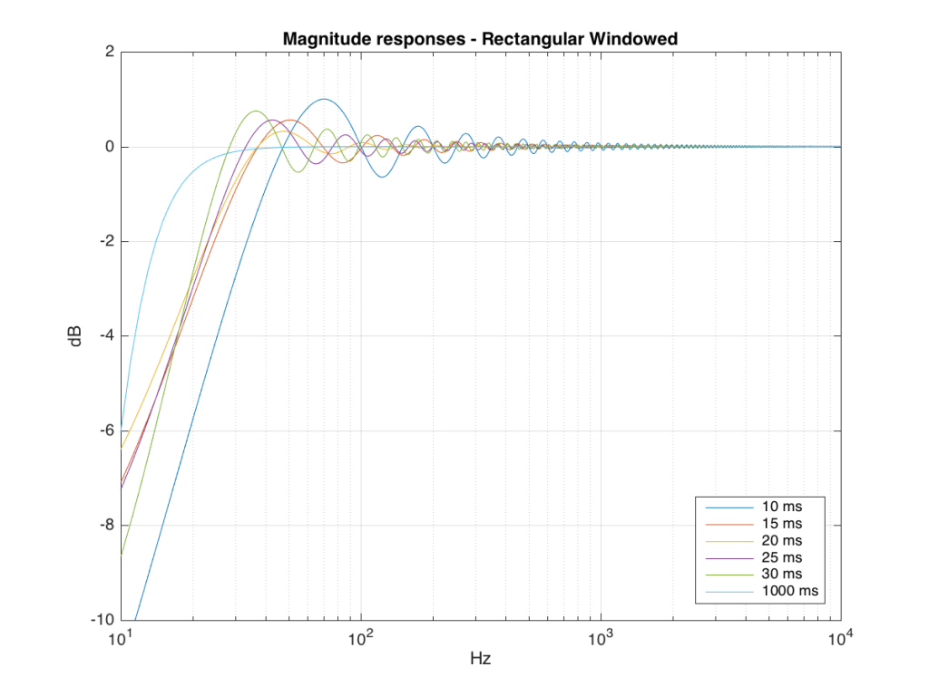
Figure 11: The magnitude responses resulting from taking an FFT of a shortened portion of a single impulse response plotted in Figure 8.
We’ll assume that the light blue curve in Figure 9 is the “reference” since, although it has some error due to the fact that the impulse response is “only” one second long, that error is very small. You can see in the dark blue curve that, by doing an FFT on only the first 10 ms of the total impulse response, we get a strange behaviour in the result. The first is that we’ve lost a lot in the low frequency region (notice that the dark blue curve is below the light blue curve at 10 Hz). We also see a strange bump at about 70 Hz – which is the beginning of a “ripple” in the magnitude response that goes all the way up into the high frequency region.
The amount of error that we get – and the specific details of how wrong it is – are dependent on the length of the portion of the impulse response that we use.
If we plot this as an error – how wrong is each of the curves relative to our reference, the result looks like Figure 12.
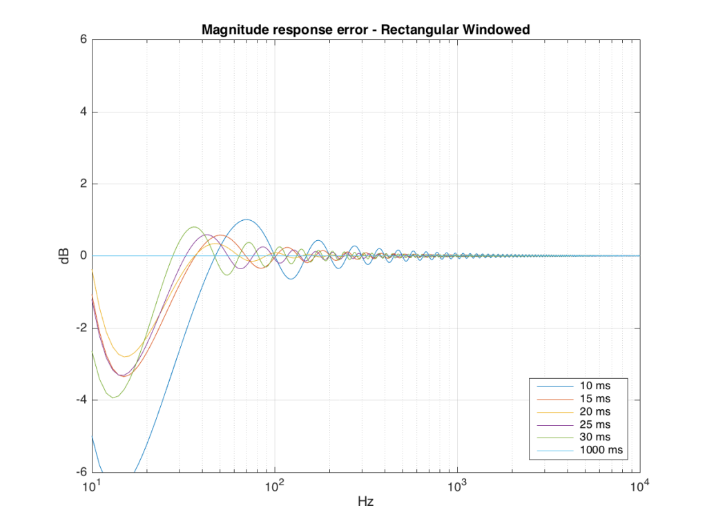
As you can see there, using a shorted impulse response produces an error in our measurement when the signal has a significant low frequency output. However, as we said above, we shorten the impulse response to delete the early reflections from the walls of The Cube in our measurement to make it “pseudo-anechoic”. This means, therefore, that we must have some error in our measurement. In fact, this is true – we do have some error in our measurement – but the error is smaller than it would have been if the room had been smaller. A bigger room means that we can have a longer impulse response which, in turn, means that we have a more accurate magnitude response measurement.
“So why not use an anechoic chamber and not mess around with this ‘pseudo-anechoic’ stuff?” I hear you cry… This is a good idea, in theory – however, in practice, the problem that we see above is caused by the fact that the loudspeaker has a low-frequency output. Making a room anechoic at a very low frequency (say, 10 Hz) would be very expensive AND it would have to be VERY big (because the absorptive wedges on the walls would have to be VERY deep – a good rule of thumb is that the wedges should be 1/4 of the wavelength of the lowest frequency you’re trying to absorb, and a 10 Hz wave has a wavelength of 34.4 m, so you’d need wedges about 8.6 m deep on all surfaces… This would therefore be a very big room…)
Of course, there are some tricks that can be played to make the room seem bigger than it is. One trick that we use is to do our low-frequency measurements in the “near field” which is much closer than 3 m from the loudspeaker, as is shown in Figure 13 below. The advantage of doing this is that it makes the direct sound MUCH louder than the wall reflections (in addition to making the difference in their time of arrival at the microphone slightly longer) which reduces their impact on the measurement. The problem with doing near-field measurements is that you are very sensitive to distance – and you typically have to assume that the loudspeaker is radiating omnidirectional – but this is a fairly safe assumption in most cases.

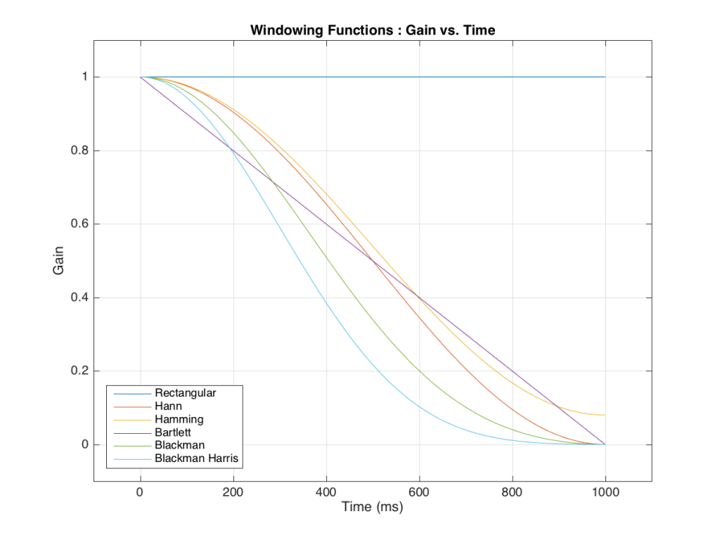
Those of you with some experience with FFT’s may have heard of something called a windowing function which is just a fact way to slice up the impulse response. Instead of either letting signal through or not, we can choose to “fade out” the impulse response more gradually. This changes the error that we’ll get, but we’ll still get an error, as can be seen below.
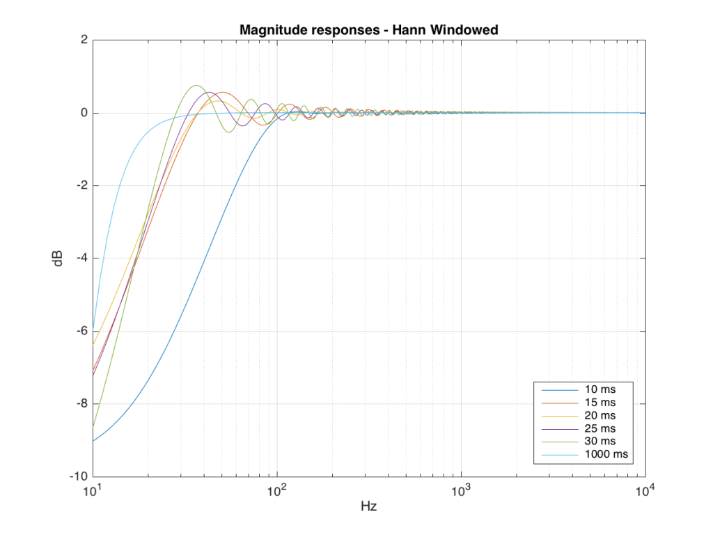
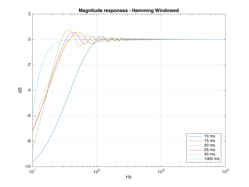
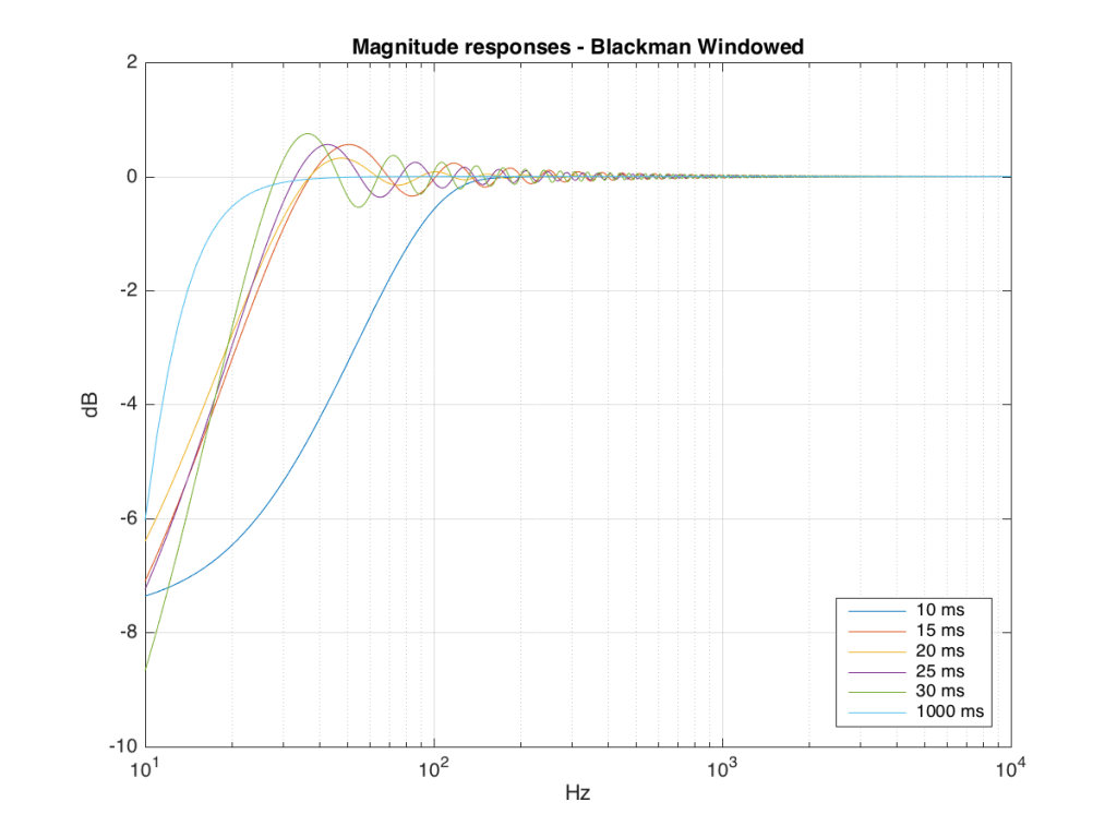
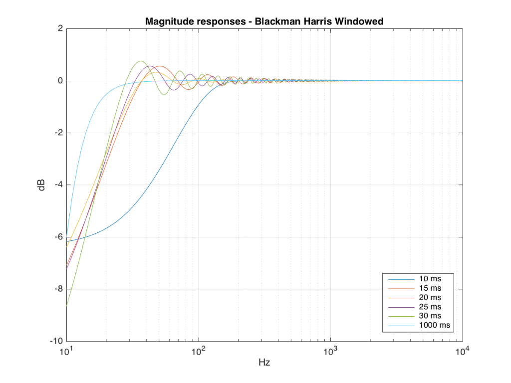
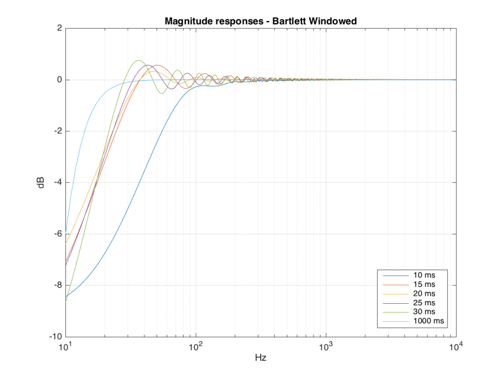
So, as you can see with all of those, the error is different for each windowing function and impulse response length – but there’s no “magic bullet” here that makes the problems go away. If you have a loudspeaker with low-frequency output, then you need a longer impulse response to see what it’s doing, even in the higher frequencies.