This one is actually by request, but I was reminded that it’s one of my pet peeves as well.
The nice thing about this one is that someone else has written about this topic, so I don’t have to do it.
This one is actually by request, but I was reminded that it’s one of my pet peeves as well.
The nice thing about this one is that someone else has written about this topic, so I don’t have to do it.
Yesterday, I once again read something on the Internet by someone saying something like “of course, as you know, high frequency sound travels faster than low frequencies”.
This is not true for any practical purposes within the limits of human hearing.
The speed of sound in air, in m/s is approximately
331.67 + 0.607*Temperature
So, at 20°C, the speed of sound is just under 344 m/s. I normally say 345 m/s, partly because 22°C is a good guess, and it’s easier to type.
Any dependency on frequency is measurable, but should not be considered to be perceivable – and is certainly not worth laying awake at night, worrying about it. There is a small, easily ignored (about 0.1 m/s) increase in the speed going up to 100 Hz, and then it’s pretty constant from there up.
Sometimes, on a rare occasion, I can muster up enough gumption to admit that I’m wrong. This posting is just such an admission…
Once-upon-a-time, I learned about equal loudness contours (I will explain these below…). Then I learned about weighting filters and how they’re used to make a measurement system as imperfect as we are. (I will also explain this below). The short explanation at the end of that lesson was “A-weighting is for measuring quiet sounds, and C-weighting is for loud sounds.”
This put a hard-and-fast belief in my head that then made me grumpy any time someone published a specification that said something like “maximum sound pressure level: 120 dB SPL (A)”, since 120 dB SPL is NOT a quiet sound – so the idiot that wrote that should have used a C-weighting instead.
However, as Bertrand Russell once said, “It’s healthy now and then to hang a question mark on things you’ve long taken for granted.” It turns out that my almost-religious-indignation regarding “mis-” use of weighting curves might not be so righteous after all.
Once-upon-a-time, some research (Fletcher and Munson) figured out that humans do not have a flat frequency response. We are, generally speaking, more sensitive to midrange information than lower- and higher-frequency bands. If you a play a tone for a test subject at a given sound pressure level at 1 kHz, then change to a different frequency and ask the subject to adjust the level of the second frequency so that it sounds the same level as the 1 kHz tone, you get some offset gain value. If you do that again and again for a lot of frequencies and a lot of people and average the results, you get curves that show contours of equal loudness – the sound pressure levels of different frequencies that sound the same level to us.
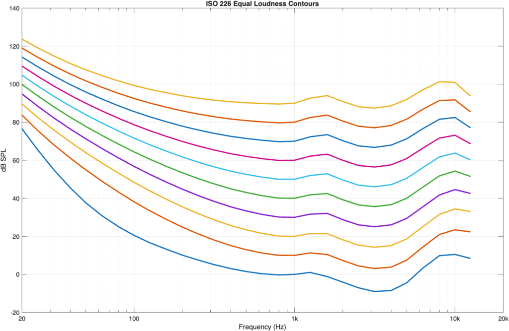
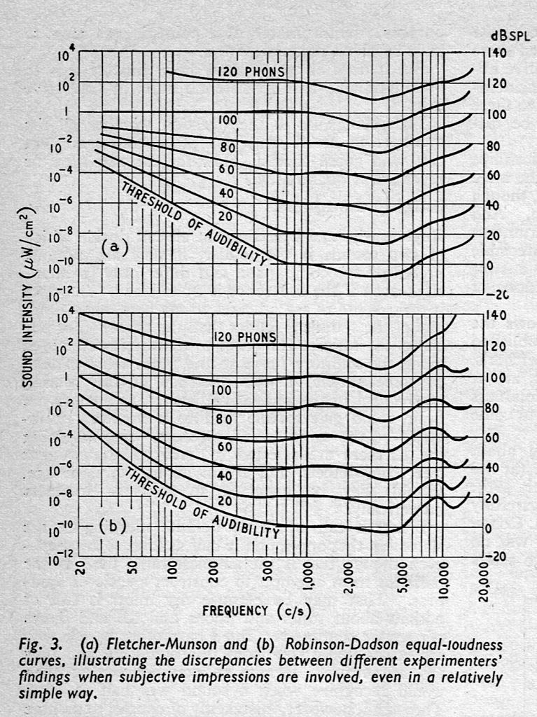
Figure 1, above shows the ISO 226 version of these equal loudness contours which are more like the ones found by Robinson and Dadson and not Fletcher and Munson, as can be seen in the comparison of the two data sets, below.
The curves are typically labelled using the SPL value where they cross 1 kHz. For example, the curve that hits 50 dB SPL at 1 kHz is called the “50-phon” curve; a sinusoidal tone at a given frequency on that line will have a perceived loudness of 50 phons, which will be 50 dB SPL at only 3 frequencies, one of which is 1 kHz.
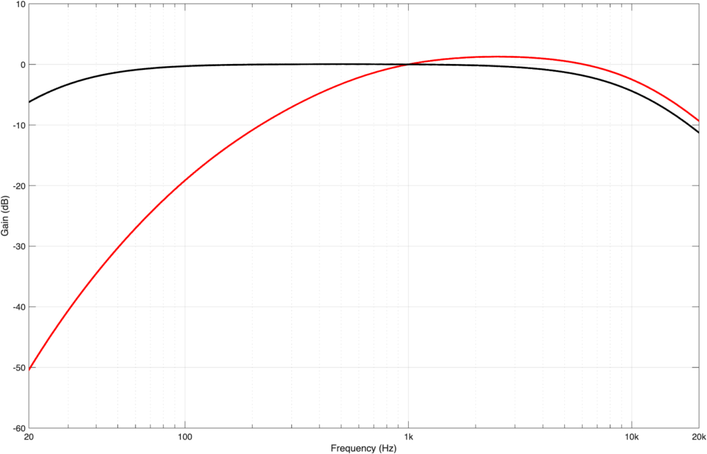
As I mentioned above, the A- and C-weighting filters (as well as other variants) were designed to simulate this lack-of-linearity to make measurements (like noise levels, for example) more aligned with human perception. For example, as can be seen above, we are bad at hearing low frequencies at low levels. So, if you are tasked with measuring the background noise caused by an air conditioning system in an office space, you’ll bring a microphone that can detect the noise better than we can, which results in you getting a high SPL value for something that we can’t hear. Therefore, we apply a roll-off to the microphone’s output before capturing a measurement value. This is the purpose of an A-weighting filter, the response of which is shown in Figure 3, below.
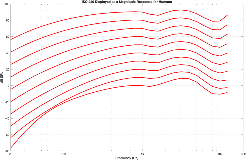
If we flip the equal loudness contours upside-down so that they show our hearing sensitivity as a magnitude response, then they’d look like the curves in Figure 4.
If you read the Wikipedia page on A-weighting you’ll come across these two statements:
The A-weighting was based on the 40-phon Fletcher–Munson curves, which represented an early determination of the equal-loudness contour for human hearing.
Subsequent research has demonstrated that A-weighting is in closer agreement with the updated 60-phon contour incorporated into ISO 226:2003 than with the 40-phon Fletcher-Munson contour, which challenges the common misapprehension that A-weighting represents loudness only for quiet sounds.
Let’s then test this by plotting the A-weighting response on top of the equal loudness contours.
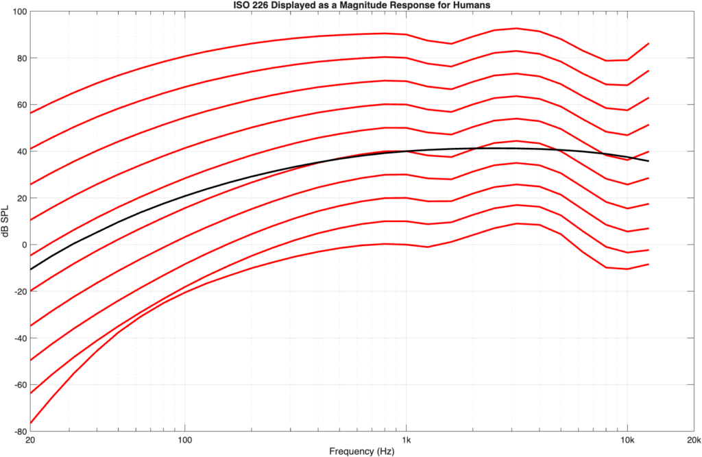
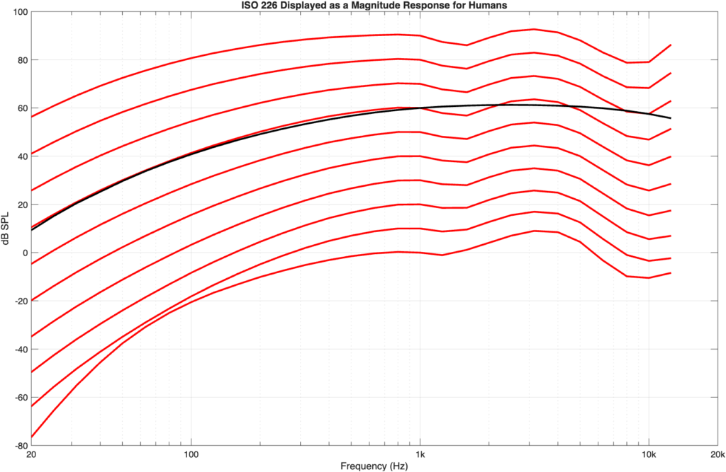
As you can see in Figure 5 and 6, the A-weighting curve better matches the 60-phon curve than the 40-phon curve. If I do this more generally, by looking at the difference between the A-weighting curve and each of the equal loudness contours (viewed as a magnitude response) then the result is as shown in Figure 7.
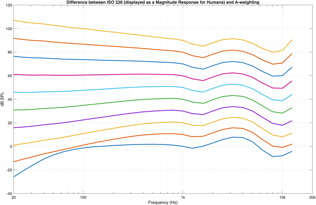
As you can see there, the flattest curve is the one for 60-phon; the one that crosses 1 kHz at 60 dB SPL, so that statement from Wikipedia is correct.
Of course, 60 dB SPL is not THAT loud – and it’s certainly not the same as 120 dB SPL… but it seems that my high horse might not be worth staying on, and maybe using A-weighting as a general approximation, regardless of the level might NOT be as terrible a sin as I believed for so many years…
Mea culpa
Once-upon-a-time, I taught a course in electroacoustic measurements at McGill. I used to devote an entire 3-hour class to explaining decibels, partly because we use them so often in audio, partly because I had such difficulty wrapping my own head around them when I was starting off, and partly because the reason I and many other people have that problem is largely due to the laziness of others.
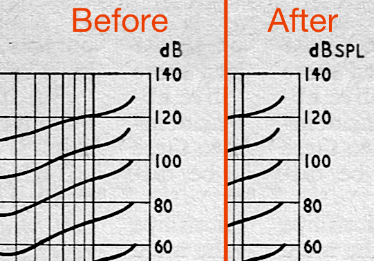
Yesterday, I found myself being annoyed once again by this laziness as I edited a scan of a document from 1961 to correct it before posting it online…
Some background information:
We humans generally respond to things logarithmically. Without getting into the math, this means that our reptile brains like multiplication more than addition.
For example: if I have $10 in the bank, and you have $100 – and we both win $10 in a lottery, I’ll be happier than you. We both won the same amount of money, but I won 100% of my current balance, whereas you only won 10% of your current balance.
Another example is a piano keyboard. Each octave looks the same distance on the keyboard, but the fundamental frequency of those notes are doubling each time you go up one octave. So, a piano keyboard (and music notation) are frequencies displayed on a logarithmic scale.
This is also true of detecting how loud things are: we think “twice as loud” or “half as loud” when talking about the Sound Pressure Level (SPL) that we hear.
We use percent and octaves to do two things:
When it comes to comparing levels of things like Sound Pressure Level, electrical power, voltages, or radio signal power, we use decibels (or dB) to make the scale logarithmic.
So, you’ll see someone write something like “the sound of a jet engine at takeoff is 120 decibels”, which is when my pet peeve rears its ugly head. The problem is that this sentence is incomplete.
If you do the math, then you find out that “120 decibels” is the same as saying “1,000,000 times” (because 10^(120/20) = 1,000,000)*, which means that the following two sentence fragments say exactly the same thing:
“louder than” what? THIS is the problem. The sentence should have said
“the sound of a jet engine at takeoff is 120 dB SPL” which means
“the sound of a jet engine at takeoff is 1,000,000 times louder than the quietest level that an average person can hear when the audio signal is a 1 kHz sinusoidal tone.”
Without the “SPL” after the “dB”, there’s no way to know what you’re talking about, which is why, 40 years ago, I couldn’t understand what a “decibel” was – and why, 10 years later, my students had such trouble as well.
Without the “SPL”, it would be like if speed limits said that you should drive “50 km/”. Per second? Per minute? Per hour? Per day? These are very different things…
This also means that if you’re talking about something else, then you need a different letter after the “dB”. For example:
and there are lots more…
In case it’s interesting, a before-and-after of the plot that I edited yesterday is here:
… and if you want to dig into this a little more deeply, then I wrote this explanation for my electroacoustic measurements course 30 years ago
* Five last things:
#1: If you already have the measurement of the thing that you want to express in decibels relative to something else, AND it’s a pressure or voltage measurement, then the math you do is:
x dB = 20 * log10(Pressure1 / Pressure2)
For example, if Pressure1 = 2.5 pascals and Pressure2 = 1.25 pascals, then
20 * log10(2.5/1.25) = 6.02 dB
So you can say that 2.5 pascals is 6.02 decibels higher than 1.25 pascals.
If, instead, Pressure2 is the standard reference of 20 µPa, then:
20 * log10(2.5/0.00002) = 101.9
So, you can say that 2.5 pascals is 101.9 dB SPL.
#2: If you want to do it backwards for pressure or voltage then the math you do is:
Pressure2 * 10^(dB/20) = Pressure1
If you have the dB SPL value and you want to find out how many pascals you’re talking about, then Pressure2 = 0.00002
For example, if you know that the measurement is 101.9 dB SPL, then:
0.00002 * 10^(101.9 / 20) = 2.489 pascals
#3: Some examples:
#4: If you’re measuring power (in electrical watts or acoustic watts), then the math is slightly different.
#5: If you also see a letter in parentheses at the end such as dB SPL (A) or dB SPL (C), then this means something that you cannot ignore, but that I will not explain here…
#105 in a series of articles about the technology behind Bang & Olufsen loudspeakers
I’ve started working with a number of my colleagues on a series of videos for internal training at Bang & Olufsen. They were kind enough to make some of these videos publicly available.
This video explains why loudspeaker drivers are typically put in enclosures (boxes), the three types of enclosures that we use (sealed, ported, and passive radiators), and the differences in impact that these enclosure types have on the loudspeaker’s behaviour.
#104 in a series of articles about the technology behind Bang & Olufsen loudspeakers
I’ve started working with a number of my colleagues on a series of videos for internal training at Bang & Olufsen. They were kind enough to make some of these videos publicly available.
This video explains the various components inside a typical loudspeaker driver.
#103 in a series of articles about the technology behind Bang & Olufsen loudspeakers
I’ve started working with a number of my colleagues on a series of videos for internal training at Bang & Olufsen. They were kind enough to make some of these videos publicly available.
This one explains why loudspeaker drivers produce a narrower “beam” of sound at higher frequencies and how multiple loudspeaker drivers can be used to control both the direction and the width of an acoustic beam.
#102 in a series of articles about the technology behind Bang & Olufsen loudspeakers
I’ve started working with a number of my colleagues on a series of videos for internal training at Bang & Olufsen. They were kind enough to make some of these videos publicly available.
This video explains (and demonstrates) how recording engineers are able to control the perceived location of different sound sources in a two-channel stereo recording using different techniques.
#101 in a series of articles about the technology behind Bang & Olufsen loudspeakers
I’ve started working with a number of my colleagues on a series of videos for internal training at Bang & Olufsen. They were kind enough to make some of these videos publicly available.
This video explains how we are able to localise the direction of and the distance to a sound source in the real world.
Note that there are two small errors in the video. I said that 800 µsec is 8 millionths of a second. It’s 800 millionths of a second. I’ll let you find the other error.
#100 in a series of articles about the technology behind Bang & Olufsen loudspeakers
I’ve started working with a number of my colleagues on a series of videos for internal training at Bang & Olufsen. They were kind enough to make some of these videos publicly available.
This one explains some basic concepts of human hearing in the frequency domain, including how our hearing changes with level, the reason we use “loudness” processing in loudspeakers, and psychoacoustic masking.
In case you’re interested in looking into this a little further, the curves I show there are from the Robinson-Dadson experiments, not the Fletcher-Munson version. An interesting place to start learning about the history of this is the March, 1962 issue of Wireless World magazine, which includes this plot comparing the two.