In this posting, we’ll do something similar to the analyses from Part 7. In that one, we
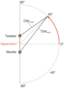
- took two point-source theoretically perfect loudspeaker drivers (which means that they have the same magnitude response in all directions in 3D space), (pretending that they were a tweeter and a woofer in a non-existent cabinet)
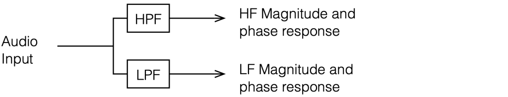
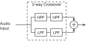
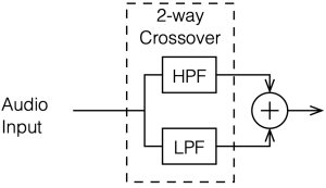
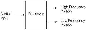
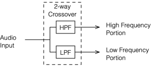
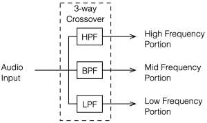
- filtered each of their inputs using a crossover network
- separated them by some distance
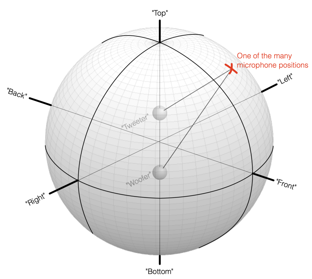
- measured them in a bunch of places on a sphere surrounding the non-existent cabinet
- found the total magnitude response of the system when measured all around on that sphere, which is called the loudspeaker’s Power Response.
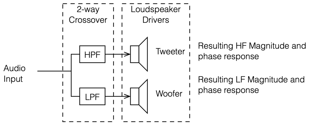
Now, we do that again, but we will include the real loudspeaker drivers’ measurements in that three-dimensional world. In this case, we still have the 1″ tweeter and the 6″ woofer in a sealed cabinet. Those two loudspeaker drivers were individually measured at 130 points around them on that sphere that I showed in Part 7.
I then take each of those 130 measurements for each driver, filter them using the crossover, and add the two outputs together, which gives me the magnitude response of the entire loudspeaker with two drivers for each individual location. We then add the 130 measurements to find a total combined response which is the Power Response of the two-way loudspeaker with two real loudspeaker drivers in a real cabinet, with the 5 different crossover types that we’ve been talking about.
Note that I have NOT done what I said I SHOULD do at the end of part 9. I have just been dumb and stuck the crossovers in front of the loudspeaker drivers without thinking about modifying the filters to compensate for the drivers’ characteristics.
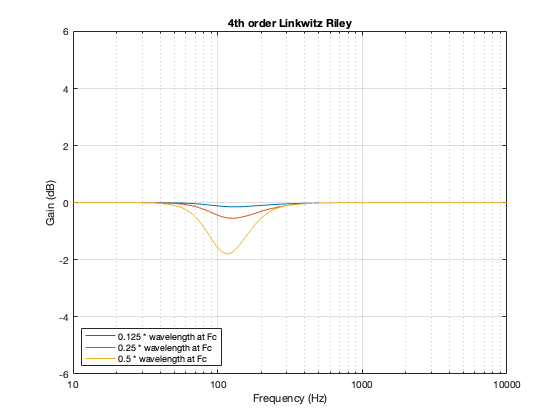
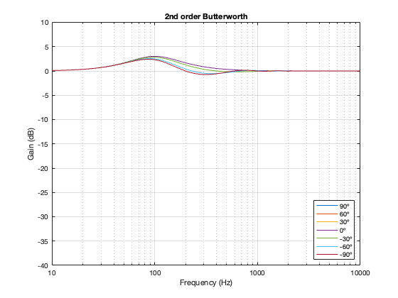
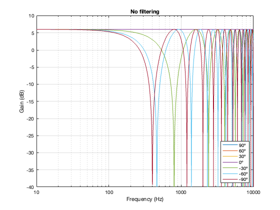
The five resulting power responses are shown in Figure 10.1.
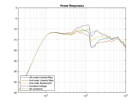
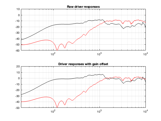
The first thing to notice is that there is a roll-off in the low end. This is the natural response of the woofer that we saw in Part 9.
The second thing that you’ll notice is the general downward-slope in the top octave of the plot, starting at about 7 kHz and having a generally decreasing magnitude the higher you go in frequency. This is the result of “beaming”. Since the two loudspeaker drivers, generally, have less and less high-frequency output as you move off-axis, then this appears as less total output from the system on that sphere. If the two loudspeakers were omnidirectional, then the power response would be a horizontal line. The more directional the drivers, the steeper the downward slope of this plot.
The last thing that’s easy to see in this plot is the transition between the woofer and the tweeter. It appears as that steep slope just above 1 kHz. Remember that I put the crossover at 1.8 kHz – so the slope doesn’t sit right on the crossover frequency. But it’s easy to see that something is happening to the directivity of the loudspeaker in that area.
Now remember back to Part 7, where we did a little trick where we made an assumption that a person building or installing a loudspeaker would measured its on-axis response, and then put in an equaliser to flatten this measured response.
In the old days, you would do this “by eye” using something like a graphic or a parametric equaliser. But nowadays, we have fancy tools that can do measurements and create complicated FIR filters that do whatever we want. This means that we can REALLY screw things up with the precision of a surgical scalpel…
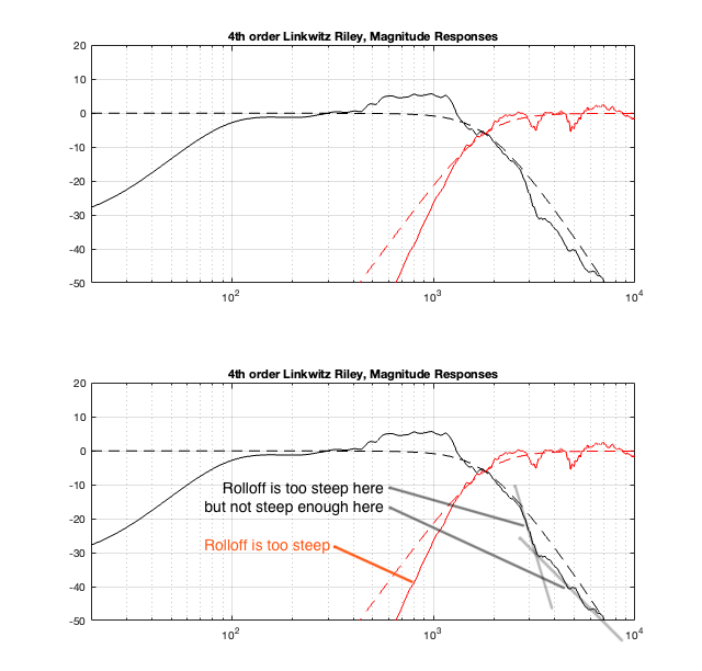
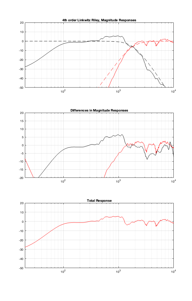
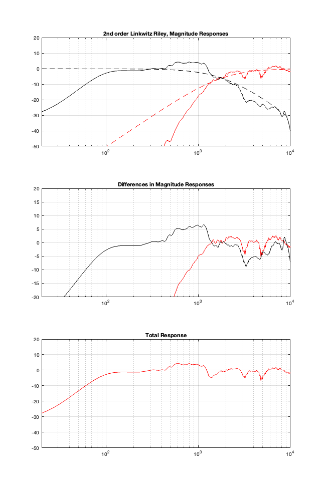
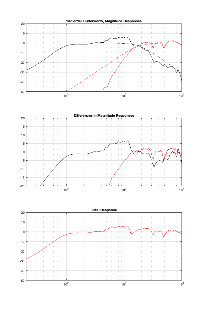
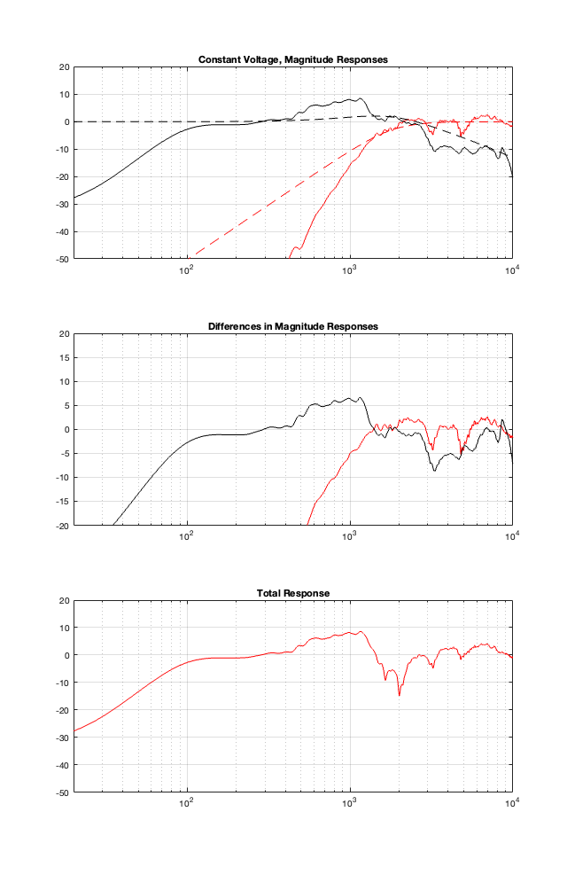
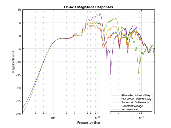
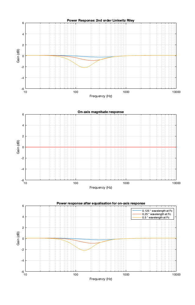
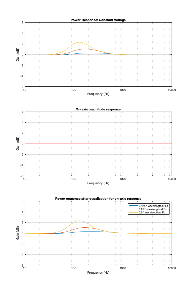
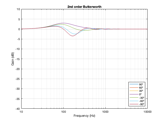
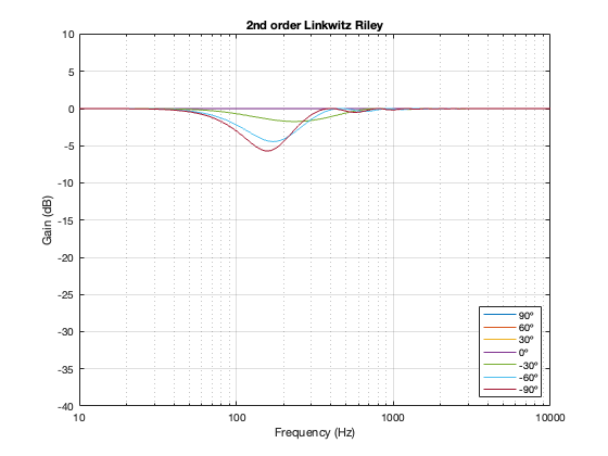
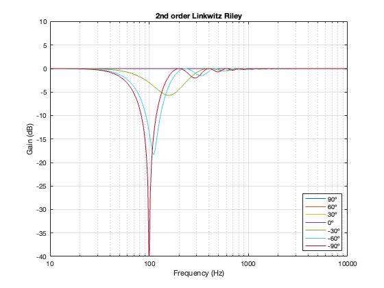
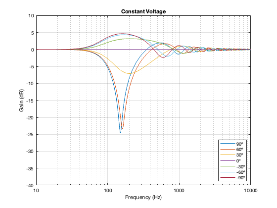
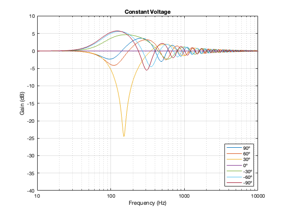
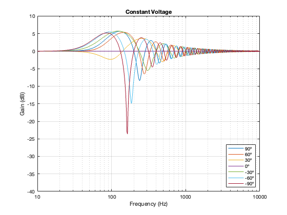
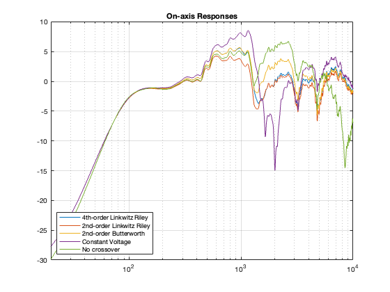
So, let’s be dumb and do the same thing again. We’ll take the on-axis responses of the loudspeaker with the different crossovers (we already saw these in Part 9, but here they are again, shown in Figure 10.2), and we’ll make five “perfect” equalisers that make each of these five responses perfectly flat.
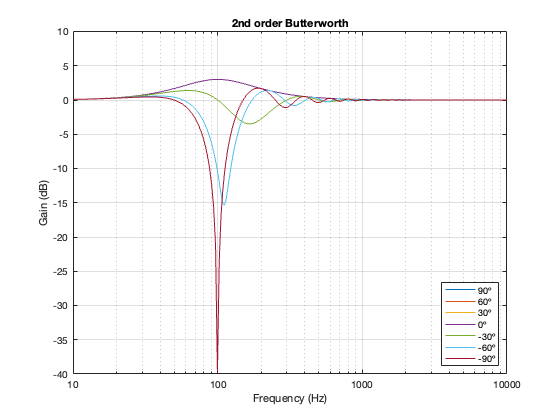
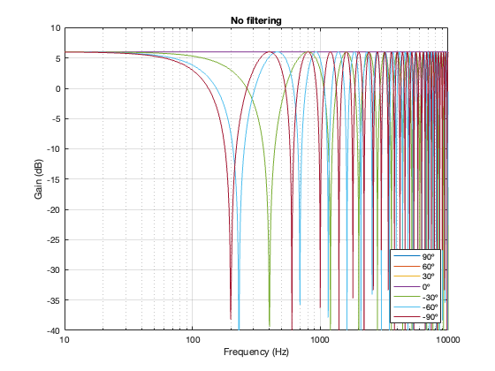
After applying each of these customised filters that make our on-axis measurement look like a laser beam, we should probably check what happened to the power responses. They’re shown below in Figure 10.3.
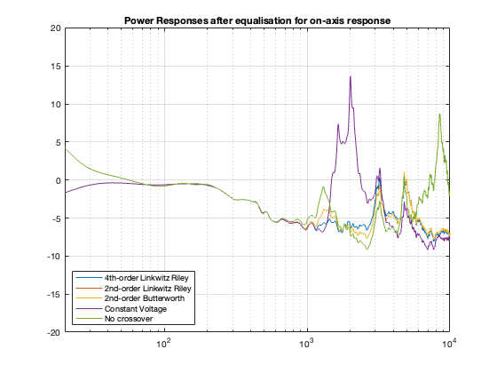
As you can see there, the low frequency response flattens out. This is because we’re really boosting the bass (to fix the on-axis measurement) and this loudspeaker happens to be fairly omnidirectional below about 200 Hz.
You can also see that I was REALLY dumb when I made those equalisation filters. For example, the notch in the on-axis response of the Constant Voltage caused me to make a horrendous peak that results in a really nice-looking plot at one on-axis point in space, but completely messes up the response of the loudspeaker in almost all other directions, resulting in that giant 15 dB peak around 2 kHz (remember that our crossover frequency is in this region…). I also wound up pushing up the low end by something like 30 dB, which is nuts.
The moral of this story is “don’t fix the on-axis response without considering the power response”. OR “just because it looks flat doesn’t mean that it’ll sound good.” On the other hand, notice that, after equalisation, most of the other curves look pretty similar-ish which means that maybe doing some intelligent equalisation for the on-axis response isn’t necessarily a bad idea.
Remember, however, that we’re still only looking at the loudspeaker in infinite space. There’s no room “singing along” with this loudspeaker… but the topic of room compensation is for another time…
N.B. About a week after I made this posting, I found an error in my Matlab code that calculated the plots. They’ve now been updated to the correct curves. The conclusions listed in the text haven’t changed, but some of the little details have.
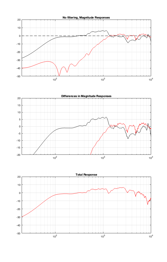
Extra note for the sake of transparency
Figure 10.3 was made using a method that is about as stupid and lazy as I could have possibly done. For each crossover type, all I did was to subtract the values shown in the plot in Figure 10.2 from those in Figure 10.1. This is probably not the way that you would implement a “flattening” filter in real life, but it is similar to the old-fashioned strategy used by systems that blindly make an FIR filter based on a single measurement.