B&O Tech: Where great sound starts

#25 in a series of articles about the technology behind Bang & Olufsen loudspeakers


You’ve bought your loudspeakers, you’ve connected your player, your listening chair is in exactly the right place. You sit down, put on a new recording, and you don’t like how it sounds. So, the first question is “who can I blame!?”

Of course, you can blame your loudspeakers (or at least, the people that made them). You could blame the acoustical behaviour of your listening room (that could be expensive). You could blame the format that you chose when you bought the recording (was it 128 kbps MP3 or a CD?). Or, if you’re one of those kinds of people, you could blame the quality of the AC mains cable that provides the last meter of electrical current supply to your amplifier from the hydroelectric dam 3000 km away Or you could blame the people who made the recording.

In fact, if the recording quality is poor (whatever that might mean) then you can stop worrying about your loudspeakers and your room and everything else – they are not the weakest link in the chain.

So, this week, we’ll talk about who those people are that made your recording, how they did it, and what each of them was supposed to look after before someone put a CD on a shelf (or, if you’re a little more current, put a file on a website).


Recording Engineer

The recording engineer is the person you picture of when you think about a recording session. You have the musicians in the studio or the concert hall, singing and playing music. That sound travels to microphones that were set up by a Recording Engineer who then sits behind a mixing console (if you’re American – a “mixing desk” if you’re British) and fiddles with knobs obsessively.

Fig 1. A recording engineer (the gentleman on the right) engineering a recording. This is actually probably a staged shot – but it could easily have been taken either during the tracking or mixing part of the process.

There’s a small detail here that we should not overlook. Generally speaking, a “recording engineer” has to do two things that happen at different times in the process of making a recording. The first is called “tracking” and the second is called “mixing”.


Tracking

Normally, bands don’t like playing together – sometimes because they don’t even like to be in the same room as each other.  Sometimes schedules just don’t work out. Sometimes the orchestra and the soloist can’t be in the same city at the same time.

In order to circumvent this problem, the musicians are recorded separately in a process called “tracking”. During tracking, each musician plays their part, with or without other members of the band or ensemble. For example, if you’re a rock band, the bass and the drummer usually arrive first, and they play their parts. In the old days, they would have been recorded to seaport tracks on a very wide (2″!) magnetic tape (hence the term “tracking”) where each instrument is recorded on a separate track. That way, the engineer has a separate recording of the kick drum and the snare drum and each tom-tom and each cymbal, and so on and so on. Nowadays, most people don’t record to magnetic tape because it’s too expensive. Instead, the tracks are recorded on a hard disc on a computer. However, the process is basically the same.

Once the bass player and the drummer are done, then the guitarist comes into the studio to record his or her parts while listening to the previously-recorded bass and drum parts over a pair of headphones. Then the singer comes in and listens to the bass, drums and guitar and sings along. Then the backup vocalists come in, and so on and so on, until everyone has recorded their part.

During the tracking, the recording engineer sets up and positions the microphones to get the optimal sound for each instrument. He or she will make sure that the gain that is applied to each of those microphones is correct – meaning that it’s recorded at a level that is high enough be mask the noise floor of the electronics and the recording medium, but not so high that it distorts. In the old days, this was difficult because the dynamic range of the recording system was quite small – so they had to stay quite close to the ceiling all the time – sometimes hitting it. Nowadays, it’s much easier, since the signal paths have much wider dynamic ranges so there’s more room for error.


In the case of a classical recording, it might be a little different for the musicians, but the technical side is essentially the same. For example, an orchestra will play (so you don’t bring in the trombone section first – everyone plays together) with a lot of microphones in the room. Each microphone will be recorded on its own individual track, just like with the rock band. The only difference is that everyone is playing at the same time.
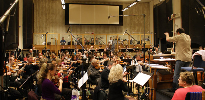
Fig 2. A typical orchestra recording session. Note that all the musicians are there, and there are a lot of microphones in the room. Each of those microphones is probably being recorded on its own independent track on a hard disc somewhere so that they can be mixed together later.


Once all the tracking is done the musicians are finished. They’ve all been captured, each on their own track that can be played back later in isolation (for example, you can listen to just the snare drum, or just the microphone above the woodwind section). Sometimes, they will even have played or sung their part more than once – so we have different versions or “takes” to choose from later. This means that there may be hundreds of tracks that all need to be mixed together (or perhaps just left out…) in order to make something that normal people can play on their stereo.


Mixing

Now that all the individual tracks are recorded, they have to be combined into a pretty package that can be easily delivered to the customers. This means that all of those individual tracks that have been recorded have to be assembled or “mixed” together into a version that has, say, only two channels – one for the left loudspeaker and one for the right loudspeaker. This is done by feeding each individual track to its own input on a mixing console and listening to them individually to see how they best fit together. This is called the “mixing” process. During this stage, basic decisions are made like “how loud should the vocals be relative to the guitars (and everything else)”. However, it’s a little more detailed than that. Each track will need its own processing or correction (maybe changing the equalisation on the snare drum – or altering the attack and decay of the bass guitar using a dynamic range compressor – or the level of the vocal recording is changed throughout the tune to compensate for the fact that the singer couldn’t stay the same distance from the microphone whilst singing…) that helps it to better fit into the final mix.

Fig 3. A mixing console that has been labelled with the various tracks for the input strips. This is a very typical look for a console during a mixing session – although the surroundings are not.


If you walk into the control room of a recording studio during a mixing session, you’d see that it looks almost exactly like a recording session – except that there are no musicians playing in the studio. This is because what you usually see on videos like this one is a tracking session – but the recording engineer usually does a “rough mix” during tracking – just to get a preliminary idea of how the puzzle will fit together during mixing.

Once the mixing session for the tune is finished, then you have a nearly-finished product. You at least have something that the musicians can take home to have a listen to see if they’re satisfied with the overall product so far.


Editing

In classical music there is an extra step that happens here. As I said above, with classical recordings, it’s not unusual for all the musicians to play in the same room at the same time when the tracking is happening. However, it is unusual that they are able to play all the way through the piece without making any mistakes or having some small issues that they want to fix. So, usually, in a classical recording, the musicians will play through the piece (or the movement) all the way through 2 or 3 times. While that happens, a Recording Producer is sitting in the control room, listening and making notes on a copy of the score. Each time there is a mistake, the producer makes a note of it – usually with a red make indicating the Take Number in which the mistake was made. If, after 2 or 3 full takes of the piece, there are points in the piece that have not been played correctly, then they go back and fix small bits. The ensemble will be asked to play, say 5 bars leading up to the point that needs fixing – and to continue playing for another 5 bars or so.

Later, those different takes (either full recordings, or bits and pieces) will be cut and spliced together in a process called editing. In the old days, this was done using a razor blade to cut the magnetic tape and stick it back together. For example, if you listen to some of Glen Gould’s recordings, you can hear the piano playing along, but the tape hiss changes suddenly in the background noise. This is the result of a splice between two different recordings – probably made on different days or with different brands of tape. Nowadays, the “splicing” is done on a computer where you fade out of one take and fade into another gradually over 10 ms or so.

Fig 4. A “crossfade” on a modern digital audio workstation. The edit point (what used to be a “tape splice”) is where the recording on the top right is faded out and a different recording (bottom right) of the same music is faded in.


If the editing was perfect, then you’ll never hear that it happened. Sometimes, however, it’s possible to hear the splice. For example, listen to this recording and  listen to the overall level and general timbre of the piano. It changes to a quieter, duller sound from about 0′ 27″ to about 0´ 31″. This is a rather obvious tape splice to a different recording than the rest of the track.


Mastering Engineer

The final stage of creating a recording is performed by a Mastering Engineer in a mastering studio. This person gets the (theoretically…) “finished” product and makes it better. He or she will sit in a room that has very little gear in it, listening to the mixed song to hear if there are any small things that need fixing. For example, perhaps the overall timbre of the tune needs a little brightening or some control of the dynamic range.

Another basic role of the mastering engineer is to make sure that all of the tracks on a single album sound about the same level – since you don’t want people sitting at home fiddling with the volume knob from tune to tune.

When the mastering engineer is done, and the various other people have approved the final product, then the recording is finished. All that is left to do is to send the master to a plant to be pressed as a CD – or uploaded to the iTunes server – or whatever.


Fig 5. A mastering engineer sitting at a mastering console. Notice that, unlike a mixing console, a mastering console does not have a massive number of faders and knobs because it doesn’t have a lot of inputs. Also note that the mastering engineer looks better rested and more cleanly shaven than the recording engineer (above) because he doesn’t have to talk to musicians every day at work. Okay, okay, I’m joking… sort of…


In other words the Mastering Engineer is the last person to make decisions about how a recording should sound before you get it.

This is why, when I’m talking to visitors, I say that our goal at Bang & Olufsen is to build loudspeakers that perform so that you, in your listening room, hear what the mastering engineer heard – because the ultimate reference of how the recording should sound is what it sounded like in the mastering studio.


Appendicies

What’s a producer?

The title of Recording Producer means different things for different projects. Sometimes, it’s the person with the money who hires everyone for the recording.

Sometimes (usually in a pop recording) it’s the person sitting in the control room next to the recording engineer who helps the band with the arrangement – suggesting where to put a guitar solo or where to add backup vocals. Some pop producers will even do good ol’ fashioned music arrangements.

A producer for a classical recording usually acts as an extra set of ears for the musicians through the recording process. This person will also sit with the recording engineer in the control room, following the score to ensure that all sections of the piece have been captured to the satisfaction of the performers. He or she may also make suggestions about overall musical issues like tempi, phrasing, interpretation and so on.


But what about film?

The basic procedure for film mixing is the same – however, the “mixing engineer” in a film world is called a “re-recording engineer”. The work is similar, but the name is changed.


So that’s a “Tonmeister”?

A tonmeister is a person who can act simultaneously as a Recording Engineer and a Recording Producer. It’s a person who has been trained to be equally competent in issues about music (typically, tonmeisters are also musicians), acoustics, electronics, as well as recording and studio techniques.


B&O Tech: How loud are my headphones?

As you may already be aware, Bang & Olufsen makes headphones: the BeoPlay H6 over-ear headphones and the BeoPlay H3 earbuds.

If you read some reviews of the H6 you’ll find some reviewers like them very much and say things like  “…excellent clarity and weight, well-defined bass and a sense of openness and space unusual in closed-back headphones. The sound is rich, attractive and ever-so-easy to enjoy.” and “… by no means are these headphones designed only for those wanting a pounding bass-line and an exciting overall balance: as already mentioned the bass extension is impressive, but it’s matched with low-end definition and control that’s just as striking, while a smooth midband and airy, but sweet, treble complete the sonic picture.” (both quotes are from Gramophone Magazine’s April 2014 issue). However, some other reviewers say things like “My only objection to the H6s is their volume level is not quite as loud as I normally would expect.” (A review from an otherwise-satisfied on Amazon.com). And, of course, there are the people whose tastes have been influenced by the unfortunate trend of companies selling headphones with a significantly boosted low-frequency range, and who now believe that all headphones should behave like that. (I sometimes wonder if the same people believe that, if it doesn’t taste like a Big Mac, it’s not a good burger… I also wonder why they don’t know that it’s possible to turn up the bass on most playback devices… But I digress…)

For this week’s posting, I’ll just deal with the first “complaint” – how loud should a pair of headphones be able to play?

Part 1: Sensitivity

One of the characteristics of a pair of headphones, like a passive loudspeaker, is its sensitivity. This is basically a measurement of how efficient the headphones are at converting electrical energy into acoustical output (although you should be careful to not confuse “Sensitivity” with “Efficiency” – sensitivity is a measure of the sound pressure level or SPL output for the voltage at the input whereas efficiency is a measure of the SPL output for the power in milliwatts). The higher the sensitivity of the headphones, the louder they will play for the same input voltage.

So, if you have a pair of headphones that are not very sensitive, and you plug them into your smartphone playing a tune at full volume, it might be relatively quiet. By comparison, a pair of very sensitive headphones plugged into the same smartphone playing the same tune at the same volume might be painfully loud. For example,let’s look at the measured data for three not-very-randomly selected headphones at https://www.stereophile.com/content/innerfidelity-headphone-measurements.

BrandModelVrms to produce 90 dB SPLdBV to produce 90 dB SPL
SennheiserHD6000.230-12.77
BeoplayH60.044-27.13
EtymoticER4PT0.03-30.46

If we do a little math, this means that, for the same input voltage, the Etymotic’s will be 3.3 dB louder than the H6’s and the Sennheiser’s will be 14.4 dB quieter. This is a very big difference. (The Etymotic’s are 7.7 times louder than the Sennheisers!)

So, in other words, different headphones have different sensitivities. Some will be quieter than others – some will be louder.

Side note: If you want to compare different pairs of headphones for output level, you could either look them up at the stereophile.com site I mentioned above, or you could compare their data sheet specifications using the Sensitivity to Efficiency converter on this page.

The moral of this first part of the story is that, when someone says “these headphones are not very loud” – the question is “compared to what?”

Part 2: The Source

I guess it goes without saying, but if you want more out of your headphones, the easiest solution is to turn up the volume of your source. The question then is: how much output can your source deliver? This answer also varies greatly from product to product. For example, if I take four not-very-randomly selected measurements that I did myself, I can see the following maximum output levels for a 500 Hz,  0 dB FS sine tone at maximum volume sent to a 31 ohm load (a resistor pretending to be a pair of headphones):

BrandModelVrmsdBV
LenovoThinkPad T4200.317-9.98
AppleiPhone 3Ds0.89-1.01
AppleMacBook Pro2.085+6.38
SonyCDP-D5006.69+16.51

In other words, the Sony is more than 26 dB (or 21 times) louder than the ThinkPad, if we’re just measuring voltage. This is a very big difference.

So, as you can see, turning the volume all the way up to 11 on different product results in very different output levels. This is even true if you compare iPod Nano’s of different generations, for example – no two products are the same.

The moral of the story here is: if your headphones aren’t loud enough, it might not be the headphones’ fault.

Part 3: The Details, French Law, and How to Cheat

So much for the obvious things – now we are going to get a little ugly.

Let’s begin the ugliness with a little re-hashing of a previous posting. As I talked about in this posting, your ears behave differently at different listening levels. More specifically, you don’t hear bass and treble as well when the signal is quiet. The louder it gets, the more flat your “frequency response”. This means that, when acoustical consultants are making measurements of quiet things, they usually have to make the microphone signal as “bad” as your hearing at low levels. For example, when you’re measuring air conditioning noise in an office space, you want to make your microphone less sensitive to low frequencies, otherwise you’ll get a reading of a high noise level when you can’t actually hear anything. In order to do this, we use something called an “weighting filter” which is an attempt to simulate your frequency response. There are many different weighting curves – but the one we’ll talk about in this posting is an “A-weighting” curve. This  is a filter that attenuates the low and high frequencies and has a small boost in the mid-band – just like you do at quiet listening levels. The magnitude response of that curve is shown below in Figure 1. At higher levels (like measuring the noise level at the end of a runway while a plane is taking off over your head), you might want to use a different weighting curve like a “C-weighting” filter – or none at all.

The magnitude response of an A-weighting filter.
Fig 1. The magnitude response of an A-weighting filter.

So, let’s say that you get enough money on Kickstarter to create the Fly-by-Night Headphone Company and you’re going to make a flagship pair of headphones that will sweep the world by storm. You do a little research and you start coming across something called “BS EN 50332-1” and “BS EN 50332-2“. Hmmmm… what are these? They’re international standards that define how to measure how loudly a pair of headphones plays. The procedure goes something like this:

  1. get some pink noise
  2. filter it to reduce the bass and the treble so that it has a spectrum that is more like music (the actual filter used for this is quite specific)
  3. reduce its crest factor so your measurement doesn’t jump around so much (this basically just gets rid of the peaks in the signal)
  4. do a quick check to make sure that, by limiting the crest factor, you haven’t changed the spectrum beyond the acceptable limits of the test procedure
  5. play the signal through the headphones and measure the sound pressure level using a dummy head
  6. apply an A-weighting to the measurement
  7. calculate how loud it is (averaged over time, just to be sure)

So, now you know how loud your headphones can play using a standard measurement procedure. Then you find out that, according to another international standard called EN 60065 or EN 60950-1 there are maximum limits to what you’re permitted to legally sell… in France… for now… (Okay, okay, these are European standards, but Europe has more than one country in it, so I think that I can safely call them international…)

So, you make your headphones, you make them sound like you want them to sound (I’ll talk about the details of this in a future posting), and then you test them (or have them tested) to see if they’re legal in France. If not (in other words, if they’re too sensitive), then you’ll have to tweak the sensitivity accordingly.

Okay – that’s what you have to do – but let’s look at that procedure a little more carefully.

Step 1 was to get some pink noise. This is nothing special – you can get or make pink noise pretty easily.

Step 2 was to filter the noise so that its spectrum ostensibly better matches the average spectrum of all recorded and transmitted music and speech in the world. The details of this filter are in another international standard called IEC 60268-1.  The people who wrote this step mean well – there’s no point in testing your headphones with frequencies that are outside the range of anything you’ll ever hear in them. However, this means that there is probably some track somewhere that includes something that is not represented by the spectral characteristics of the test signal we’re using here. For example: Figure 2, below shows the spectral curve of the test signal that you are supposed to send to the headphones for the test.

The magnitude response of the filter applied to the pink noise before sending it to the headphones.
Fig 2. The magnitude response of the filter applied to the pink noise before sending it to the headphones.

Compare that to Figure 3, which shows an analysis of a popular Lady Gaga tune that I use as part of my collection of tunes to make a woofer unhappy. This is a commercially-available track that has not been modified in any way.

The spectrum of a Lady Gaga tune. Compare this with the noise filter plot from Figure 2 (plotted in red for your convenience).
Fig 3. The spectrum of a Lady Gaga tune. Compare this with the noise filter plot from Figure 2 (plotted in red for your convenience).

As you can see, there is more energy in the music example than there is in the test signal around the 30 – 60 Hz octave – particularly noticeable due to the relative “hole” in the response that ranges between about 70 and 700 Hz.

Of course, if we took LOTS of tunes and analysed them, and averaged their analyses, we’d find out that the IEC test signal shown in Figure 2 is actually not too bad. However, every tune is different from the average in some way.

So, the test signal used in the EN 50332 test is not going to push headphones as hard as some kinds of music (specifically, music that has a lot of bass content),

We’ll skip Step 3, Step 4, and Step 5.

Step 6 is a curiosity. We’re supposed to take the signal that we recorded coming out of the headphones and apply an A-weighting filter to it. Now, remember from above that an A-weighting filter reduces the low and high frequencies in an effort to simulate your bad hearing characteristics at quiet listening levels. However, what we’re measuring here is how loud the headphones can go. So, there is a bit of a contradiction between the detail of the procedure and what it’s being used for. However, to be fair, many people mis-use A-weighting filters when they’re making noise measurements. In fact, you see A-weighted measurements all the time – regardless of the overall level of the noise that’s being measured. One possible reason for this is that people want to be able to compare the results from the loud measurements to the results from their quiet ones – so they apply the same weighting to both – but that’s just a guess.

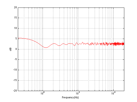
Let’s, just for a second, consider the impact of combining Steps 2 and 6. Each of the filters in both of these steps reduce the sensitivity of the test to the low and high frequency behaviour of the headphones. If we combine their effects into a single curve, it looks like the one in Figure 4, below.

The magnitude response of the combination of the A-weighting filter and the filter applied to the pink noise signal.
Fig 4. The magnitude response of the combination of the A-weighting filter and the filter applied to the pink noise signal.

At this point, you may be asking “so what?” Here’s what.

Let’s take two different pairs of headphones and pretend that we measured them using the procedure I described above. The first pair of headphones (we’ll call it “Headphone A”) has a completely flat frequency response +/- < 0.000001 dB from 20 Hz to 20 kHz. The second pair of headphones has a bass boost such that anything below about 120 Hz has a 20 dB gain applied to it (we’ll call that “Headphone B”). The two unweighted measurements of these two simulated headphones are shown in Figure 5.

The magnitude responses of the two simulated headphones. The blue curve is "Headphone A". The red curve is "Headphone B".
Fig 5. The magnitude responses of the two simulated headphones. The blue curve is “Headphone A”. The red curve is “Headphone B”.

After filtering these measurements with the weighting curves from Steps 2 and 6 (above), the way our measurement system “hears” these headphone responses is slightly different – as you can see in Figure 6, below.

The magnitude responses of the two simulated headphones as "seen" by a EN 50332 measurement. The blue curve is "Headphone A". The red curve is "Headphone B".
Fig 6. The magnitude responses of the two simulated headphones as “seen” by a EN 50332 measurement. The blue curve is “Headphone A”. The red curve is “Headphone B”.

So, what happens when we measure the sound pressure level of the pink noise through these headphones?

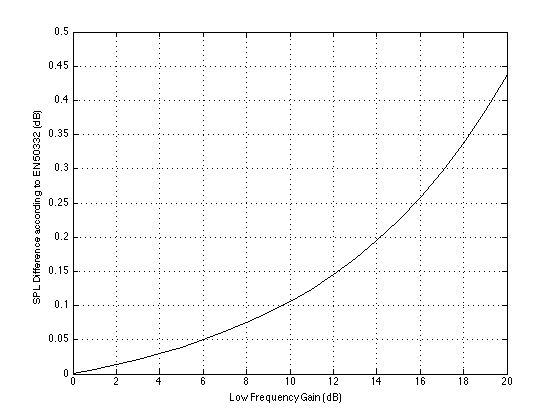
Well, if we did the measurements without applying the two weighing curves, but just using good ol’ pink noise and no messin’ around, we’d see that Headphone B plays 13.1 dB louder than Headphone A (because of the 20 dB bass boost). However, if we apply the filters from Steps 2 and 6, the measured difference drops to only 0.46 dB.

This is interesting, since the standard measurement “thinks” that a 20 dB boost in the entire low frequency region corresponds to only a 0.46 dB increase in overall level.

Figure 7 shows the relationship between the bass boost applied below 120 Hz and the increase in overall level as measured using the EN 50332 standard.

The relationship between the increase in SPL as measured using the EN 50332 standard vs. the gain of a bass boost applied to the headphones. (filter characteristics are Low shelving, fc=120 Hz, Q=0707)
Fig 7. The relationship between the increase in SPL as measured using the EN 50332 standard vs. the gain of a bass boost applied to the headphones. (filter characteristics are Low shelving, fc=120 Hz, Q=0.707)

So, let’s go back to you, the CEO of the Fly-by-Night Headphone Company. You want to make your headphones louder, but you also need to obey the law in France. What’s a sneaky way to do this? Boost the bass! As you saw above, you can crank up the bass by 20 dB and the regulators will only see a 0.46 dB change in output level. You can totally get away with that one! Some people might complain that you have too much bass in your headphones, but hey – kids love bass. And plus, your competitors will get complaints about how quiet their headphones are compared to yours. All because people listening to children’s records at high listening levels hear much more bass than the EN 50332 measurement can!

Of course, one other way is to just ignore the law and make the headphones louder by increasing their sensitivity… but no one would do that because it’s illegal. In France.

Appendix 1: Listen to your Mother!

My mother always told me “Turn down that Walkman! You’re going to go deaf!” The question is “Was my mother right?” Of course, the answer is “yes” – if you listen to a loud enough sound for a long enough time, you will damage your hearing – and hearing damage, generally speaking, is permanent.  The louder the sound, the less time it takes to cause the damage. The question then is “how loud and how long?” The answer is different for everyone, however you can find some recommendations for what’s probably safe for you at sites that deal with occupational health and safety. For example, this site lists the Canadian recommendations for maximum exposure time limits to noise in the workplace. This site shows a graph for the US recommendations for the same thing – I’ve used the formula on that site to make the graph in Figure 8, below.

Recommendations for the maximum time of exposure to noise sources according to The National Institute for Occupational Safety and Health (NIOSH) in the USA.
Fig 8. Recommendations for the maximum time of exposure to noise sources according to The National Institute for Occupational Safety and Health (NIOSH) in the USA.

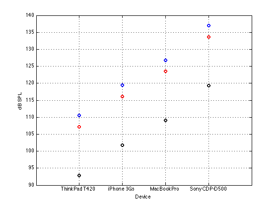
How do these noise levels compare with what comes out of my headphones? Well, let’s go back to the numbers I gave in Part 1 and Part 2. If we take the measured maximum output levels of the 4 devices listed in Part 2, and calculate what the output level in dB SPL would be through the measured sensitivities of the headphones listed in Part 1 (assuming that everything else was linear and nothing distorted or clipped or became unhappy – and ignoring the fact that the headphones do not have the same impedance as the one I used to do the measurements of the 4 devices… and assuming that the measurements of the headphones are unweighted on that website), then the maximum output level you can get from those devices are shown in Figure 9.

Calculated maximum output levels in dB SPL for the four devices and three headphones listed in Parts 1 and 2, above.
Fig 9. Calculated maximum output levels in dB SPL for the four devices and three headphones listed in Parts 1 and 2, above. Blue is the Etymotic ER4PT, red is the BeoPlay H6, and black is the Sennheiser HD600.

So, if you take the calculations shown in Figure 8 and compare them to the recommendations shown in Figure 7, then you might reach the conclusion that, if you set your volume to maximum (and your tune is full-band pink noise mastered to a constant level of  0 dB FS, and we do a small correction for the A-weighting based on the assumption that the 90 dB SPL headphone measurements listed above are unweighted ), then the maximum recommended time that you should listen to your music, according to the federal government in the USA is as shown in Figure 10.

Recommended maximum exposure time for 3 different headphones connected to 4 different sources playing at maximum volume.
Fig 10. Recommended maximum exposure time for 3 different headphones connected to 4 different sources playing at maximum volume (based on a large number of assumptions that may or may not be correct).

So, if I only listen to full-bandwidth pink noise at 0 dB FS at maximum volume on my MacBook Pro over my BeoPlay H6’s, then the American government thinks that after 0.1486 of a second, I am damaging my hearing.

It seems that my mother was right.

Appendix 2: Why does France care about how loud my headphones are?

This is an interesting question, the answer to which makes sense to some people, and doesn’t make any sense at all to other people – with a likely correlation with your political beliefs and your allegiance to the Destruction of the Tea in Boston. The best answer I’ve read was discussed in this forum where one poster very astutely point out that, in France, the state pays for your medical care. So, France has a right to prevent the French from making themselves go deaf by listening to this week’s top hit on Spotify at (literally) deafening levels. If you live in a place where you have to pay for your own medical care, then you have the right to self-harm and induce your own hearing impairment in order to appreciate the subtle details buried within the latest hip-hop remix of Mr. Achy-Breaky Heart’s daughter “singing” Wrecking Ball while you’re riding on a bus. In France, you don’t.

Appendix 3: Additional Reading

ISVR Consulting’s page

Rodhe and Schwarz’s pdf manual for running the EN 50332 test on their equipment

B&O Tech: Visual Analogies to Problems in Audio

#23 in a series of articles about the technology behind Bang & Olufsen loudspeakers


Audio people throw words around like “frequency” and “distortion” and “resolution” and “” without wondering whether anyone else in the room (a) understands or (b) cares. One of the best ways to explain things to people who do not understand but do care is to use analogies and metaphors. So, this week, I’d like to give some visual analogies of common problems in audio.


Let’s start with a photograph. Assuming that your computer monitor is identical to mine, and the background light in your room is exactly the same as it is in mine, then you’re seeing what I’m seeing when you look at this photo.

original

Let’s say that you, sitting there, looking at this photo is analogous to you, sitting there, listening to a recording on a pair of loudspeakers or over headphones. So what happens when something in the signal path messes up the signal?


Perhaps, for example, you have a limited range in your system. That could mean that you can’t play the very low and/or high frequencies because you are listening through a smaller set of loudspeakers instead of a full-range model. Limiting the range of brightness levels in the photo is similar to this problem – so nothing is really deep black or bright white. (We could have an argument about whether this is an analogy to a limited dynamic range in an audio system, but I would argue that it isn’t – since audio dynamic range is limited by a noise floor and a clipping level, which we’ll do later…) So, the photo below “sounds” like an audio system with a limited range:

limited_range

Of course, almost everything is there – sort of – but it doesn’t have the same depth or sparkle as the original photo.


Or what if you have a noisy device in your signal chain For example, maybe you’re listening to a copy of the recording on a cassette tape – or the air conditioning is on in your listening room. Then the result will “sound” like this:

noise

As you can see, you still have the original recording – but there is an added layer of noise with it. This is not only distracting, but it can obscure some of the more subtle details that are on the same order of magnitude as the noise itself.


In audio, the quietest music is buried in the noise of the system (either the playback system or the recording system). On the other extreme is the loud music, which can only go so loud before it “clips” – meaning that the peaks get chopped off because the system just can’t go up enough. In other words, the poor little woofer wants to move out of the loudspeaker by 10 mm, but it can only move 4 mm because the rubber holding on to it just can’t stretch any further. In a photo, this is the same as turning up the brightness too much, resulting in too many things just turning white because they can’t get brighter (in the old days of film, this was called “blowing out” the photo), as is shown below.

clipping


This “clipping” of the signal is what many people mean when they say “distorted” – however, distortion is a much broader range of problems then just clipping. To be really pedantic, any time the output of a system is not identical to its input, then the signal is distorted.


A more common problem that many people face is a modification of the frequency response. In audio, the frequency is (very generally speaking) the musical pitch of the notes you’re hearing. Low notes are low frequencies, high notes are high frequencies. Large engines emit low frequencies, tiny bells emit high frequencies. With light, the frequency of the light wavicle hitting your eyeball determines the colour that you see. Red is a low frequency and violet is a high frequency (see the table on this page for details). So, if you have a pair of headphones that, say, emphasises bass (the low frequencies) more than the other areas, then it’s the same as making the photo more red, as shown below.

freq_response


Of course, not all impairments to the audio signal are accidental. Some are the fault of the user who makes a conscious decision to be more concerned with convenience (i.e. how many songs you can fit on your portable player) than audio quality. When you choose to convert your CD’s to a “lossy” format (like MP3, for example), then (as suggested by the description) you’re losing something. In theory, you are losing things that aren’t important (in other words, your computer thinks that you can’t hear what’s thrown away, so you won’t miss it). However, in practice, that debate is up to you and your computer (and your bitrate, and the codec you’ve chosen, and the quality of the rest of your system, and how you listen to music, and what kind of music you’re listening to, and whether or not there are other things to listen to at the same time, and a bunch of other things…) However, if we’re going to make an analogy, then we have to throw away the details in our photo, keeping enough information to be moderately recognisable.

limited_res

As you can see, all the colours are still there. And, if you stand far enough away (or if you take off your glasses) it might just look the same. But, if you look carefully enough, then you might notice that something is missing… Keep looking… you’ll see it…


So, as you can see, any impairment of the “signal” is a disruption of its quality – but we should be careful not to confuse this with reality. There are lots of people out there who have a kind of weird religious belief that, when you sit and listen to a recording of an orchestra, you should be magically transported to a concert hall as if you were there (or as if the orchestra were sitting in your listening room). This is silly. That’s like saying when you sit and watch a re-run of Friends on your television, you should feel like you’re actually in the apartment in New York with a bunch of beautiful people. Or, when you watch a movie, you feel like you’re actually in a car chase or a laser battle in space. Music recordings are no more of a “virtual reality” experience than a television show or a film. In all of these cases (the music recording, the TV episode and the film), what you’re hearing and seeing should not be life-like – they should be better than life. You never have to wait for the people in a film to look for a parking space or go out to pee. Similarly, you never hear a mistake in the trumpet solo in a recording of  Berlin Philharmonic and you always hear Justin Bieber singing in tune. Even the spatial aspects of an “audiophile” classical recording are better-than-reality. If you sit in a concert hall, you can either be close (and hear the musicians much louder than the reverberation) or far (and hear much more of the reverberation). In a recording, you are sitting both near and far – so you have the presence of the musicians and the spaciousness of the reverb at the same time. Better than real life!

So, what you’re listening to is a story. A recording engineer attended a music performance, and that person is now recounting the story of what happened in his or her own style. If it’s a good recording engineer, then the storytelling is better than being there – it’s more than just a “police report” of a series of events.

To illustrate my point, below is a photo of what that sinking WWII bunker actually looked like when I took the photo that I’ve been messing with.

reality


Of course, you can argue that this is a “better” photo than the one at the top – that’s a matter of your taste versus mine. Maybe you prefer the sound of an orchestra done recorded with only two microphones played through two loudspeakers. Maybe you prefer the sound of the same orchestra recorded with lots of microphones played through a surround system. Maybe you like listening to singers who can sing. Maybe you like listening to singers who need auto tuners to clean up the mess. This is just personal taste. But at least you should be choosing to hear (or see) what the artist intended – not a modified version of it.

This means that the goal of a sound system is to deliver, in your listening room, the same sound as the recording engineer heard in the studio when he or she did the recording. Just like the photos you are looking at on the top of this page should look exactly the same as what I see when I see the same photo.


B&O Tech: Listening Tips & Tricks

#22 in a series of articles about the technology behind Bang & Olufsen loudspeakers


Let’s say that you go to the store and you listen to a pair of loudspeakers with some demo music they have on a shelf there, and you decide that you like the loudspeakers, so you buy them.

Then, you take them home, you set them up, and you put one of your recordings, and you change your mind – you don’t like the loudspeakers.

What happened? Well, there could be a lot of reasons behind this.


Tip #1: Loudness

In the last article, I discussed why a “loudness” function is necessary when you change the volume setting while listening to your system. The setup of this article discussed the issue of Equal Loudness Contours, shown again as a refresher in Figure 1, below.

Fig 2: The Equal Loudness contours for 0 phons (bottom curve) to 90 phons (top curve) in 10 phone increments, according to ISO226.
Fig 1: The Equal Loudness contours for 0 phons (bottom curve) to 90 phons (top curve) in 10 phon increments, according to ISO226.

Let’s say that, when you heard the loudspeakers at the store, the volume knob was set so that, if you had put in a -20 dB FS, 1 kHz sine wave, it would have produced a level of  70 dB SPL at the listening position in the store. Then, let’s say that you go home and set the volume such that it’s about 10 dB quieter than it was when you heard it at the store. This means that, even if you listen to exactly the same recording, and even if your listening room at home were exactly the same as the room at the store, and even if the placement of the loudspeakers and the listening position in your house were exactly the same as at the store, the loudpspeakers would sound different at home than at the store.

Figure 2 below shows the difference between the 70 phon curve from Figure 1 (sort of what you heard at the store) and the 60 phon curve (sort of what you hear at home, because you turned down the volume). (To find out which curve is which in Fig 1, the phon value of the curve is its value at 1 kHz.)


Fig 2:
Fig 2: The normalised difference between the 60 phon curve and the 70 phon curve from Fig 1.


As you can see in Figure 2, by turning down the volume by 10 dB, you’ve changed your natural sensitivity to sound – you’re as much as 5 or 6 dB less sensitive to low frequencies and also less sensitive to the high end by a couple of dB. In other words, by turning down the volume, even though you have changed nothing else, you’ve lost bass and treble.

In fact, even if you only turned down the volume by 1 dB, you would get the same effect, just by a different amount, as is shown in Figure 3.


Fig 3: The difference between the 67 (red), 68 (blue), and 69 (black) phon curve and the 70 phon curve. Note that these have been normalised to remove the frequency-independent gain differences. Only frequency-dependent sensitivity differences are shown.


So, as you can see here, even by changing the volume knob by 1 dB, you change the perceived frequency response of the system by about 0.5 dB in a worst case. The quieter you listen, the less bass and treble you have (relative to the perceived level at 1 kHz).

So, this means that, if you’re comparing two systems (like the loudspeakers at the store and the loudspeakers at home, or two different DAC’s or your system before and after you connect the fancy new speaker wire that you were talked into buying), if you are not listening at exactly the same level, your hearing is not behaving the same way – so any differences you hear may not be a result of the system.

Looking at this a different way, if you were to compare two systems (let’s say a back-to-back comparison of two DAC’s) that had frequency response differences like the ones shown in Figure 3, I would expect that you might expect that you could hear the difference between them. However, this is YOUR frequency response difference, just by virtue of the fact that you are not comparing them at the same listening level. The kicker here is that, if the difference in level is only 1 dB, you might not immediately hear one as being louder than the other – but you might hear the timbral differences between them… So, unless you’ve used a reliable SPL meter to ensure that they’re they same level, then they’re probably not the same level – unless you’re being REALLY careful – and even then, I’d recommend being more careful than that.

This is why, when researchers are doing real listening tests, they have to pay very careful attention to the listening level. And, if the purpose of the listening test is to compare two things, then they absolutely must be at the same level. If they aren’t, then the results of the entire listening test can be thrown out the window – they’re worthless.

It’s also why professionals who work in the audio industry like recording engineers, mastering engineers, and re-recording engineers always work at the same listening level. This, in part, ensures that they have consistency in their mixes – in other words, they have the same bass-midrange-treble balance in all their recordings, because they were all monitored at the same listening level.

Tip #2: Recordings

If you were selling your house, and you got a call from your real estate agent that there were some potential buyers coming tomorrow to see your place, you would probably clean up. If you were really keen, not only would you clean up, but you would put out some fresh flowers in a vase, and, a half-an-hour before your “guests” arrived, you’d be pulling a freshly-based loaf of bread out of the oven (because there’s nothing more welcoming than walking into a house that smells like freshly-baked bread…) You would NOT leave the bathroom in a mess, your bed unmade, dirty dishes in the sink, and yesterday’s dirty socks on the floor. In short, you want your house to look its best – otherwise you won’t get people through the front door (unless the price is REALLY good…)

Similarly, if you worked in a shop selling loudspeakers, part of your job is to sell loudspeakers. This means that you spend a good amount of time listening to a lot of different types of music on the loudspeakers in your shop. Over time, you’ll find that some recordings sound better than others for some reason that has something to do with the interactions between the recordings, the loudspeakers, the room’s acoustics, and your preferences. If you were a smart salesperson, you would make a note of the recordings that sound “bad” (for whatever reason) and you would not play them for potential customers that come into your store. Doing so would be the aural equivalent of leaving your dirty socks on the floor.

So, this means that, if you are the customer in the shop, listening to a pair of loudspeakers that you may or may not buy, you should remember that you’re probably going to be presented with a best-case scenario. At the very least, you should not expect the salesperson to play a recording that makes the loudspeakers sound terrible. Of course, this might mean many things. For example, it might mean that the loudspeakers are GREAT – but if they’re being used to play a really bad recording that you’ve never heard before, then you might think that the reason it sounds bad is the loudspeakers, and not the recording. So, you’ll walk out of the shop hating the loudspeakers instead of the recording.

So, the moral of the story here is simple: if you’re going to a shop to listen to a pair of loudspeakers, bring your own recordings. That way, you know what to expect – and you’ll test the loudspeakers on music that you like. Even if you bring just one CD and listen to just one song – as long as the song is one that you’ve hear A LOT, then you’re going to get a much better idea of how the loudspeakers are behaving than if you let the salesperson choose the demo music. In a perfect reality, you’ll put on your song, and your jaw will drop while you think “I’ve NEVER heard it sound this good!”.


Tip #3: Room Acoustics

It goes without saying that the acoustical behaviour of a room has a huge effect on how a loudspeaker sounds (I talked about this a lot in this posting). So does the specific placement of the loudspeakers and the listening position within a room. (I talked about this a lot in this posting). So, this also means that a pair of loudspeakers in a shop’s showroom will NOT sound the same as the same loudspeakers in your house – not even if you’ve aligned the listening levels and you’re playing the same recording. Maybe you have a strong sidewall reflection in your living room that they didn’t have in the showroom. Maybe the showroom is smaller than your living room, so the room modes are at higher frequencies and “helping out” the upper bass  instead of the lower bass. Maybe, in the showroom, the loudspeakers were quite far from the wall behind them, but in your house, you’re going to push the loudspeakers up against the wall. Any of these differences will have massive effects on the sound at the listening position.

Of course, there is only one way around this problem. If you’re buying a pair of loudspeakers, then you should talk to the salesperson about taking a demo pair home for a week or so – so that you can hear how they sound in your room. If you’re buying some other component in the audio chain that might have an impact on the sound, you should ask to take it home and try it out with your loudspeakers.

If you were buying a car, you would take it for a test drive – and you would probably get out of the parking lot of the car dealer when you did so. You have to take it out on the road to see how it feels. The same is true for audio equipment – if you can’t take it home to try it out, make sure that the shop has a good return policy. Just because it sounds good in the shop doesn’t mean that it’s going to sound good in your living room.


Tip #4: Personal Taste

I like single-malt scotch. Personally, I really like peaty, smoky scotch – other people like other kinds of scotch. There’s a good book by Michael Jackson (no, not that Michael Jackson – another Michael Jackson) that rates scotches. Personally, this is a good book for me, because, not only does he give a little background for each of the distilleries, and a description of the taste of each of the scotches in there – but he scores them according to his own personal ranking system. Luckily for me, Michael Jackson and I share a lot of the same preferences – so if he likes a scotch, chances are that I will too. So, his ranking scores are a pretty good indicator for me. However, if he and I had different preferences, then his ranking system would be pretty useless.

One of my favourite quotations is from Duke Ellington who said “If it sounds good, it is good.” I firmly believe that this is true. If you like the sound of a pair of loudspeakers, then they’re good for you. Any measurement or review in a magazine that disagrees is wrong. Of course, a measurement or a reviewer might be able to point you to something that you haven’t noticed about your loudspeakers (which may make you like them a little more or a little less…) but if you like the way they sound, then there’s no need to apologise for that.

However, remember that, when you read a review, that you are reading the words of someone who also has personal taste. Yes, he/she may have heard many more loudspeakers than you have in many more listening rooms – but they still have personal preference. And, part of that personal preference is a ranking of the categories in which a loudspeaker should perform. Personally, I divide an audio system’s (or a recording’s) qualities into 5 broad categories: 1. Timbral (tone colour), 2. Spatial (i.e. imaging and spaciousness), 3. Temporal (i.e. punch, transient response), 4. Dynamics (not just total dynamic range, but also things like short term “dynamic contrast”) and 5. Distortion & Noise. Each of these has sub-headings in my head – but the relative importance of these 5 qualities are really an issue of my personal preference (and my expectations for a given product – nobody expects an iThing dock to deliver good imaging, for example…). If your personal preference of the weighting of these 5 categories (assuming that you agree with my 5 categories) is different from mine, then we’re going to like different audio systems. And that’s okay. No problem – apart from the minor issue that, if I were a reviewer working for an audio magazine, you shouldn’t buy anything I recommend. I like sushi – you like steak – so if I recommend a good restaurant, you should probably eat somewhere else.

Of course, the fact that I will listen to different music played at a different level in a different listening room than you will might also have an effect on the difference between our opinions.


Tip #5: Close your eyes

This one is a no-brainer for people who do “real” listening tests for scientific research – but it still seems to be a mystery to people who review audio gear for a living. If you want to make a fair comparison between two pieces of audio gear, you cannot, under any circumstances, know what it is that you’re comparing. There was a perfect proof of this done by Kristina Busenitz at an Audio Engineering Society convention one year. Throughout the convention, participants were invited to do a listening test on two comparable automotive audio systems. Both were installed in identical cars, parked side-by-side. The two cars were aligned to have identical reproduction levels and you listened to exactly the same materials to answer exactly the same judgements about the systems. You had to sit in the same seat (i.e. Front Passenger side) for both tests, and you had to do the two evaluations back to back. One car had a branded system in it, the other was unbranded – made obvious by the posters hanging on the wall next to one of the cars. The cars were evaluated by lots of people over the 3 or 4 days of the convention. At the end, the results were processed and it was easily proven that the branded system was judged by a vast majority of the participants to be better than the unbranded system.

There was just one catch – every couple of hours, the staff running the test would swap the posters to the opposite wall. The two cars were actually identical. The only difference was the posters that hung outside them.

So, the vast majority of professional audio engineers agreed, in a completely “fair” test, that the car with the posters (which was the opposite car every couple of hours) sounded better than the one that didn’t.

Of course, what Kristina proved was that your eyes have a bigger effect on your opinion than your ears. If you see more expensive loudspeakers, they’ll probably sound better. This is why, when we’re running listening tests internally at Bang & Olufsen, we hide the loudspeakers behind an acoustically transparent, but visually opaque curtain. We can’t help but be influenced by our pre-formed opinions of products. We’ve even seen that a packing box for a (competitor’s) loudspeaker sitting outside the listening room will influence the results of a blind listening test on a loudspeaker that has nothing to do with the label on the box. (the box was a plant – just to see what would happen).

Tip #6: Are you sure?

One last thing that really should go without saying: If you’re doing a back-to-back comparison of two different aspects of an audio system, be absolutely sure that you’re only comparing what you think you’re comparing. For example, I’ve read of people who do comparisons of things like the following:

  • sending a “bitstream” vs. “PCM” from a Blu-ray or DVD player to an AVR/Surround Processor
  • PCM vs. DSD
  • “normal” resolution vs. “high-resolution” recordings

If you’re making such a comparison, and you plan on making some conclusions, be absolutely sure that the only thing that changing in your comparison is what you think you’re comparing. In the three examples I gave above, there are potentially lots of other things changing in your signal path in addition to the thing your changing. If you’re not absolutely sure that you’re only changing one thing, then you can’t be sure that the reason you might hear a difference in the things you’re comparing is due to the thing you’re comparing. (did that make sense?) For example, given the three above examples:

  • some AVR’s apply different processing to bitstream vs. PCM signals. Some use the metadata in  a bitstream, and some players don’t when they convert to PCM. So, the REASON the bitstream and the PCM signals might sound different is not necessarily because of the signals themselves, but how the gear treats them. (see this posting for more information on this)
  • Some DAC’s (meaning the chip on the circuit board inside the box that you have in your gear) apply different filters to a DSD signal than a PCM signal. Some have a different gain on the DSD signal (some “high resolution” software-based players also apply different gains to DSD and PCM signals). So, don’t just switch from DSD to PCM and think that, because you can hear a difference, that difference is the difference in DSD and PCM. It might just be your Equal Loudness Contours playing tricks on you.
  • Some DAC’s (see previous point for my current definition of “DAC”) apply different filters to signals at different sampling rates. Don’t judge two recordings you bought at different sampling rates and think that the only difference is the sampling rate. The gear that you’re using to play the files might behave differently at different rates.

And so on.

A good analogy to this is to go to a coffee shop and buy two cups of coffee – one medium roast and one dark roast. While you’re not looking, I’ll add a little sugar to the dark roast cup – and I’ll bribe the person that made your coffee to make the medium one a couple of degrees colder than the dark one. You taste both, and you decide that dark roast is better than medium roast. But is your decision valid? No. Maybe you like sugar in your coffee. Maybe you prefer hotter coffee.  Be careful how you make up your mind…


Summary

So, to wrap up, there are (at least) four things to remember when you’re shopping for audio gear:

  1. If you’re comparing systems, make sure that you’re listening at the same level.
  2. Always listen to a system using a recording with which you’re familiar – even if it’s a bad recording. Better something you know than something you don’t.
  3. Evaluate a system that you’re planning on buying in your own listening room.
  4. Don’t let anyone tell you what sounds good or bad. Ask them what they are listening to and for in a recording or a sound system – but decide for yourself what you like.
  5. If the listening test isn’t blind, it’s not worth much. Don’t even trust your own ears if you know what you’re listening to – your ears are easily fooled by your eyes and your pre-conceived notions. And you’re not alone.
  6. Be very sure that if you’re comparing two things, then the things you think you’re comparing are the only things that you’re comparing.


B&O Tech: What is “Loudness”?

#21 in a series of articles about the technology behind Bang & Olufsen loudspeakers

Part 1: Equal Loudness Contours

Let’s start with some depressing news: You can’t trust your ears. Sorry, but none of us can.

There are lots of reasons for this, and the statement is actually far more wide-reaching than any of us would like to admit. However, in this article, we’re going to look at one small aspect of the statement, and what we might be able to do to get around the problem.

We’ll begin with a thought experiment (although, for some of you, this may be an experiment that you have actually done). Imagine that you go into the quietest room that you’ve ever been in, and you are given a button to press and a pair of headphones to put on. Then you sit and wait for a while until you calm down and your ears settle in to the silence… While that’s happening you read the instructions of the task with which you are presented:

Whenever you hear a tone in the headphones in either one of your ears, please press the button.

Simple! Hear a beep, press the button. What could be more difficult to do than that?

Then, the test begins: you hear a beep in your left ear and you press the button. You hear another, quieter beep and you press the button again. You hear an even quieter beep and you press the button. You hear nothing, and you don’t press the button. You hear a beep and you press the button. Then you hear a beep at a lower frequency and so on and so on. This goes on and on at different levels, at different frequencies, in your two ears, until someone comes in the room and says “thank you, that will be all”.

While this test seems like it would be pretty easy to do, it’s a little unnerving. This is because the room that you’re sitting in is so quiet and the beeps are also so quiet that, sometimes you think you hear a beep – but you’re not sure, because things like the sound of your heartbeat, and your breathing, and the “swooshing” of blood in your body, and that faint ringing in your ears, and the noise you made by shifting in your chair are all, relatively speaking VERY loud compared to the beeps that you’re trying to detect.

Anyways, when you’re done, you’ll might be presented with a graph that shows something called your “threshold of hearing”. This is a map of how loud a particular frequency has to be in order for you to hear it. The first thing that you’ll notice is that you are less sensitive to some frequencies than others. Specifically, a very low frequency or a very high frequency has to be much louder for you to hear it than if you’re listening to a mid-range frequency. (There are evolutionary reasons for this that we’ll discuss at the end.) Take a look at the bottom curve on Figure 1, below:

The threshold of hearing (bottom curve) and the Equal Loudness contours for 70 phons (red curve) and 90 phons (top curve) according to ISO226.
Fig 1: The threshold of hearing (bottom curve) and the Equal Loudness contours for 70 phons (red curve) and 90 phons (top curve) according to ISO226.

The bottom curve on this plot shows a typical result for a threshold of hearing test for a person with average hearing and no serious impairments or temporary issues (like wax build-up in the ear canal).  What you can see there is that, for a 1 kHz tone, your threshold of hearing is 0 dB SPL (in fact, this is how 0 dB SPL is defined…) As you go lower in frequency from there, you will have to turn up the actual signal level just in order for you to hear it. So, for example, you would need to have approximately 60 dB SPL at 30 Hz in order to be able to detect that something is coming out of your headphones or loudspeakers. Similarly, you would need something like 10 dB SPL at 10 kHz in order to hear it. However, at 3.5 kHz, you can hear tones that are quieter than 0 dB SPL! It stands to reason, then, that a 30 Hz tone at 60 dB SPL and a 1 kHz tone at 0 dB SPL and a 3.5 kHz tone at about -10 dB SPL and a 10 kHz tone at about 10 dB SPL would all appear to have the same loudness level (since they are all just audible).

Let’s now re-do the test, but we’ll change the instructions slightly. I’ll give you a volume knob instead of a button and I’ll play two tones at different frequencies. The volume knob only changes the level of one of the two tones, and your task is to make the two tones the same apparent level. If you do this over and over for different frequencies, and you plot the results, you might wind up with something like the red or the top curves in Fig 1. These are called “Equal Loudness Contours” (some people call them “Fletcher-Munson Curves because the first two researchers to talk about them were Fletcher and Munson) because they show how loud different frequencies have to be in order for you to think that they have the same loudness. So, (looking at the red curve) a 40 Hz tone at 100 dB SPL sounds like it’s the same loudness as a 1 kHz tone at 70 dB SPL or a 7.5 kHz tone at 80 dB SPL. The loudness level that you think you’re hearing is measured in “phons” – and the phon value of the curve is its value in dB SPL at 1 kHz. For example, the red curve crosses the 1 kHz line at 70 dB SPL, so it’s   the “70 phon” curve. Any tone that has an actual level in dB SPL that corresponds to a point on that red line will have an apparent loudness of 70 phons. The top curve is for the 90 phons.

Figure 2 shows the Equal Loudness Contours from 0 phons (the Threshold of Hearing) to 90 phons in steps of 10 phons.

Fig 2: The Equal Loudness contours for 0 phons (bottom curve) to 90 phons (top curve) in 10 phone increments, according to ISO226.
Fig 2: The Equal Loudness contours for 0 phons (bottom curve) to 90 phons (top curve) in 10 phon increments, according to ISO226.

There are two important things to notice about these curves. The first is that they are not “flat”. In other words, your ears do not have a flat frequency response. In fact, if you were measured the same way we measure microphones or loudspeakers, you’d have a frequency response specification that looked something like “20 Hz – 15 kHz ±30 dB” or so… This isn’t something to worry about, because we all have the same problem. So, this means that the orchestra conductor asked the bass section to play louder because he’s bad at hearing low frequencies, and the recording engineer balancing the recording adjusted the bass-to-midrange-to-treble relative levels using his bad hearing, and, assuming that the recording system and your playback system are reasonably flat-ish, then hopefully, your hearing is identically bad to the conductor and recording engineer, so you hear what they want you to.

However, I said that there are two things to notice – that was just the first thing. The second thing is that the curves are different at different levels. For example, if you look at the 0 phon curve (the bottom one) you’ll see that it raises a lot more in the low frequency region than, say, the 90 phon curve (the top one) relative to their mid-range values. This means that, the quieter the signal, the worse your ability to hear bass (and treble). For example, let’s take the curves and assume that the 70 phon line is our reference – so we’ll make that one flat, and adjust all of the others accordingly and plot them so we can see their difference. That’s shown in Figure 3.
Fig 3: The Equal Loudness contours for 0 phons (bottom curve) to 90 phons (top curve) in 10 phone increments, according to ISO226. These have all been normalised to the 70 phone curve and subsequently inverted.
Fig 3: The Equal Loudness contours for 0 phons (bottom curve) to 90 phons (top curve) in 10 phon increments, according to ISO226. These have all been normalised to the 70 phon curve and subsequently inverted.

What does Figure 3 show us, exactly? Well, one way to think of it is to go back to our “recording engineer vs. you” example. Let’s say that the recording engineer that did the recording set the volume knob in the recording studio so that (s)he was hearing the orchestra with a loudness at the 70 phon line. On other words, if the orchestra was playing a 1 kHz sine tone, then the level of the signal was 70 dB SPL at the listening position – and all other frequencies were balanced by the conductor and the engineer to appear to sound the same level as that. Then you take the recording home and set the volume so that you’re hearing things at the 30 phon level (because you’re having a dinner party and you want to hear the conversation more than you want to hear Beethoven or Justin Bieber, depending on your taste or lack thereof). Look at the curve that intersects the -40 dB line at 1 kHz (the 4th one from the bottom) in Figure 3. This shows you your sensitivity difference relative to the recording engineer’s in this example. The curve slopes downwards – meaning that you can’t hear bass as well – so, your recording playing in the background will appear to have a lot less bass and a little less treble than what the recording engineer heard – just because you turned down the volume. (Of course, this may be a good thing, since you’re having dinner and you probably don’t want to be distracted from the conversation by thumpy bass and sparkly high frequencies.)

Part 2: Compensation

In order to counter-act this “misbehaviour” in your hearing, we have to change the balance of the frequency bands in the opposite direction to what your ears are doing. So if we just take the curves in Figure 3 and flip each of them upside down, you have a “perfect” correction curve showing that, when you turn down the volume by, say 40 dB (hint: look at the value at 1 kHz) then you’ll need to turn up the low end by lots to compensate and make the overall balance sound the same.

Fig 3: The Equal Loudness contours for 0 phons (bottom curve) to 90 phons (top curve) in 10 phon increments, according to ISO226. These have all been normalised to the 70 phon curve.
Fig 4: The Equal Loudness contours for 0 phons (bottom curve) to 90 phons (top curve) in 10 phon increments, according to ISO226. These have all been normalised to the 70 phon curve.

Of course, these curves shown in Figure 4 are normalised to one specific curve – in this case, the 70 phon curve. So, if your recording engineer was monitoring at another level (say, 80 phons) then your “perfect” correction curves will be wrong.

And, since there’s no telling (at least with music recordings) what level the recording and mastering engineers used to make the recording that you’re listening to right now (or the one you’ll hear after this one), then there’s no way of predicting what curve you should use to  do the correction for your volume setting.

All we can really say is that, generally, if you turn down the volume, you’ll have to turn up the bass and treble to compensate. The more you turn down the volume, the more you’ll have to compensate. However, the EXACT amount by which you should compensate is unknown, since you don’t know anything about the playback (or monitoring) levels when the recording was done. (This isn’t the same for movies, since re-recording engineers are supposed to work at a fixed monitoring level which should be the same as all the cinemas in the world… in theory…)

This compensation is called “loudness” – although in some cases it would be better termed “auto-loudness”. In the old days, a “loudness” switch was one that, when engaged, increased the bass and treble levels for quiet listening. (Of course, what most people did was hit the “loudness”switch and left it on forever.) Nowadays, however, this is usually automatically applied and has different amounts of boost for different volume settings (hence the “auto-” in “auto-loudness”). For example, if you look at Figure 5 you’ll see the various amounts of boost applied to the signal at different volume settings of the BeoPlay V1 / BeoVision 11 / BeoSystem 4 / BeoVision Avant when the default settings have not been changed. The lower the volume setting, the higher the boost.

Fig 5: The equalisation applied by the "Loudness" function at different volume settings in the BeoPlay V1, BeoVision 11, BeoSystem 3 and BeoVision Avant. Note that these are the default settings and are customisable by the user.
Fig 5: The equalisation applied by the “Loudness” function at different volume settings in the BeoPlay V1, BeoVision 11, BeoSystem 3 and BeoVision Avant. Note that these are the default settings and are customisable by the user.

Of course, in a perfect world, the system would know exactly what the monitoring levels was when they did the recording, and the auto-loudness equalisation would change dynamically from recording to recording. However, until there is meta-data included in the recording itself that can tell the system information like that, then there will be no way of knowing how much to add (or subtract).

Historical Note

I mentioned above that the extra sensitivity we have in the 3 kHz region is there due to evolution. In fact, it’s a natural boost applied to the signal hitting your eardrum as a result of the resonance of the ear canal. We have this boost (I guess, more accurately, we have this ear canal) because, if you snap a twig or step on some dry leaves, the noise that you hear is roughly in that frequency region. So, once-upon-a-time, when our ancestors were something else’s lunch, the ones with the ear canals and the resulting mid-frequency boost were more sensitive to the noise of a sabre-toothed tiger trying to sneak up behind them, stepping on a leaf, and had a little extra head start when they were running away. (It’s like the T-shirt that you can buy when you’re visiting Banff, Alberta says: “I don’t need to run faster than the bear. I just need to run faster than you.”)

As an interesting side note to this: the end result of this is that our language has evolved to use this sensitive area. The consonants in our speech – the “s” and”t” sounds, for example, sit right in that sensitive region to make ourselves easiest to understand.

Warning note

You might come across some youtube video or a downloadable file that let’s you “check your hearing” using a swept sine wave. Don’t bother wasting your time with this. Unless the headphones that you’re using (and everything else in the playback chain) are VERY carefully calibrated, then you can’t trust anything about such a demonstration. So don’t bother.

Warning note #2 – Post script…

I just saw on another website here that someone named John Duncan made the following comment about what I wrote in this article. “Having read it a couple of times now, tbh it feels like it is saying something important, I’m just not quite sure what. Is it that a reference volume is the most important thing in assessing hifi?” The answer to this is “Exactly!” If you compare two sound systems (say, two different loudspeakers, or two different DAC’s or two different amplifiers and so on… The moral of the stuff I talk about above is that, not only in such a comparison do you have to make sure that you only change one thing in the system (for example, don’t compare two DAC’s using a different pair of loudspeakers connected to each one) you absolutely must ensure that the two things you’re comparing are EXACTLY the same listening level. A different of 1 dB will have an effect on your “frequency response” and make the two things sound like they have different timbral balances – even when they don’t.

For example, when I’m tuning a new loudspeaker at work, I always work at the same fixed listening level. (for me, this is two channels of -20 dB FS full-band uncorrelated pink noise produces 70 dB SPL, C-weighted at the listening position). Before I start tuning, I set the level to match this so that I don’t get deceived by my own ears. If I tuned loudspeakers quieter than this, I would push up the bass to compensate. If I tuned louder, then I would reduce the bass. This gives me some consistency in my work. Of course, I check to see how the loudspeakers sound at other listening levels, but, when I’m tuning, it’s always at the same level.

B&O Tech: Free / Wall / Corner

#19 in a series of articles about the technology behind Bang & Olufsen loudspeakers


If you take a careful look around the connection panel of almost any Bang & Olufsen loudspeaker, you’ll find a three-position switch that is labelled something like “Free / Wall / Corner” or “F / W / C” or “Pos 1 / Pos 2 / Pos 3”. What does this do and how should you use it?

Part 1: Unreal acoustics

Let’s pretend that you have a loudspeaker that is perfectly  omnidirectional, and it is in a free field (meaning that the sound that radiates from it is free to propagate forever without hitting anything – in other words, it’s floating in infinite space). Let’s then say that we measure the magnitude response of that loudspeaker and we find out that it has a perfectly flat response from 0 Hz to infinity Hz. Remember that the source is perfectly omnidirectional, so the response will be the same regardless of which direction you measure it from. This also means that if you do a lot of magnitude response measurements around the source and average them, it will also be flat, since the  average of a whole bunch of the same thing is the same as any one of the things (i.e. the average of 5 & 5 &  5 & 5 &  5 & 5 &  5 is 5).

The average of the magnitude responses of a perfectly omnidirectional loudspeaker, measured at all points on a sphere around it.
Fig 1. The average of the magnitude responses of a perfectly omnidirectional loudspeaker, measured at all points on a sphere around it.

Now let’s divide the infinite space in half with a very large, perfectly flat wall that extends infinitely – and we’ll put it fairly close to the loudspeaker. Now, if we do a magnitude response measurement at one position, we’ll see a response that is comprised of alternating boosts and cuts as we go up in frequency. This is caused by the interference between the direct sound of the loudspeaker and its reflection off the wall. These two sounds arrive at the measurement microphone at two different times – which means that different frequencies will be separated in phase differently. The higher the frequency, the greater the phase difference between the direct and reflected sounds. And, depending on the phase at any one frequency, the result may either be constructive interference (where the two signals add) or destructive interference (where they cancel each other). If it helps, an easier way to think of this is that the wall is a mirror that results in a reflection of the loudspeaker on the other side of it. The sound that arrives at the microphone is the combination of the two loudspeakers (the real one and the one on the other side of the mirror). If we do an averaged pressure response measurement, the averaging that we have to do results in the fact that we lose the phase information in each of our individual measurements. However, each individual response that we measure has peaks and dips that affects how it adds to the other responses. In the very low frequencies the “two” loudspeakers are very close together relative to the very long wavelengths of low frequencies in air – so they add together almost perfectly. This means that the total output will be doubled at the very low end – 200% of the output (or 6 dB more) than without the wall. At very high frequencies, the outputs of the two loudspeakers add randomly – sometimes increasing, sometimes cancelling the total. The end result of this average is a messy response, but is roughly the same level as 141% (or 3 dB more) than if the wall weren’t there. (Note that the low end is 2 times louder, (because there are two “sources” – the real one and the reflected one. However, the high end is 1.41 times louder. 1,41 is the square root of 2 – the reason for this involves an explanation of power being proportional to the square of the pressure, so doubling the power results in multiplying the pressure by sqrt(2).) Take a look at Figures 2 and 3. You’ll see that the result of placing the theoretical wall near the theoretical loudspeaker is that the low end and the high end are boosted – but the low end is boosted about 3 dB more than the high end. If you compare Figures 2 and 3, you’ll see that the closer the loudspeaker is to the wall, the higher the top frequency of the “low end”.

The average of the magnitude responses of a perfectly omnidirectional loudspeaker, 30 cm from an infinitely-extending flat wall, measured at all points on a half-sphere around it.
Fig 2. The average of the magnitude responses of a perfectly omnidirectional loudspeaker, 30 cm from an infinitely-extending flat wall, measured at all points on a half-sphere around it.


The average of the magnitude responses of a perfectly omnidirectional loudspeaker, 100 cm from an infinitely-extending flat wall, measured at all points on a half-sphere around it.
Fig 3. The average of the magnitude responses of a perfectly omnidirectional loudspeaker, 100 cm from an infinitely-extending flat wall, measured at all points on a half-sphere around it.

If you divide space once more, using a second wall that is perpendicular to the first (so now your speaker is on the floor, next to a wall, for example), you are doubling the number of “loudspeakers” again. Now we have one “real” loudspeaker and 3 reflections. Let’s forget about the magnitude response at one location for now and just deal with the power response, since that’s a little less complicated. Now we have 4 times the output (or 12 dB more) in the low frequencies and, 2 times the output (or 6 dB more) in the high frequency ranges. (Notice again that the multiplier for the output in the low end is the number of loudspeakers – either real or reflected – and that the multiplier for the output in the high frequencies is the square root of that number.)
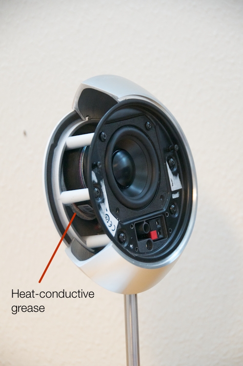
The average of the magnitude responses of a perfectly omnidirectional loudspeaker, 30 cm from each of two, perpendicular infinitely-extending flat walls, measured at all points on a quarter-sphere around it.
Fig 4. The average of the magnitude responses of a perfectly omnidirectional loudspeaker, 30 cm from each of two, perpendicular infinitely-extending flat walls, measured at all points on a quarter-sphere around it.


The average of the magnitude responses of a perfectly omnidirectional loudspeaker, 100 cm from each of two, perpendicular infinitely-extending flat walls, measured at all points on a quarter-sphere around it.
Fig 5. The average of the magnitude responses of a perfectly omnidirectional loudspeaker, 100 cm from each of two, perpendicular infinitely-extending flat walls, measured at all points on a quarter-sphere around it.


The average of the magnitude responses of a perfectly omnidirectional loudspeaker, different distances from two perpendicular infinitely-extending flat walls (30 cm and 100 cm away), measured at all points on a quarter-sphere around it.
Fig 6. The average of the magnitude responses of a perfectly omnidirectional loudspeaker, different distances from two perpendicular infinitely-extending flat walls (30 cm and 100 cm away), measured at all points on a quarter-sphere around it.

Finally, let’s add one last wall, perpendicular to the other two (i.e. two walls and the floor). This resuts in a total of 8 sources (one real and 7 reflected) which means that the output will be 8 times louder (or 18 dB) in the low end (than if the walls weren’t there) and 2.8 (sqrt(8)) times louder (or 9 dB) in the high end.

The average of the magnitude responses of a perfectly omnidirectional loudspeaker, 30 cm from each of three, perpendicular infinitely-extending flat walls, measured at all points on an eighth-sphere around it.
Fig 7. The average of the magnitude responses of a perfectly omnidirectional loudspeaker, 30 cm from each of three, perpendicular infinitely-extending flat walls, measured at all points on an eighth-sphere around it.


The average of the magnitude responses of a perfectly omnidirectional loudspeaker, 100 cm from each of three, perpendicular infinitely-extending flat walls, measured at all points on an eighth-sphere around it.
Fig 8. The average of the magnitude responses of a perfectly omnidirectional loudspeaker, 100 cm from each of three, perpendicular infinitely-extending flat walls, measured at all points on an eighth-sphere around it.

So, the first lesson to be learned here, for now, is that, in a theoretical world, where loudspeakers are perfectly omnidirectional and walls go forever, the more walls you have the bigger the bass boost. (Of course, you’ll also get a boost in the high end, but it will be smaller than the low-end boost, and you’ll probably compensate for that with the volume knob when the vocals and snare drum come in…) There is a second, nearly-as-important lesson. Look carefully, for example, at Figures 7 and 8. Starting in the low end, you can see the bass boost resulting from the collective reflections off the two walls. As you go up in frequency, you can see that the boost drops. However, before it levels out (albeit messily) at the high end, you can see that there is a deep drop in the level (i.e. in Figure 8, it’s at 100 Hz). This is because, for the particular wall distances we’re looking at, there is more cancellation of signals going on than there is constructive interference. So, the average is lower than if the walls weren’t there. This will be important later…

Part 2: Increasingly realistic acoustical behaviour

We can then take it one step further and consider that the very pretty graph shown in Figure 1 is extremely theoretical. A free field is an imaginary space – the reality is that a “free standing” loudspeaker is not really in a free field. For starters, it has to stand on something (unless you’re hanging it from the ceiling) – so the floor is not very far away – probably 1 m or so. Secondly, unless you live in a VERY large house, even when the loudspeaker is placed far from a wall, it’s probably not going to tens of metres away from any way. We can set a limit of something like 1 m on this – meaning, if you’re more than 1 m from any wall, we’ll call that “free”. This means that, in a real space, where the loudspeaker is at least 1 m from any surface, the response you get as a result of those three adjacent walls is roughly like the graph shown in Figure 8. The implications of this previous paragraph, in the real world, are important. What this means is that, when we do the sound design for a loudspeaker, we have to choose its position in a room rather carefully. Typically, it’s in a “free” position, which means, in a real world, about 1 m from each of the two adjacent walls (this isn’t measured exactly – everything in this article should be considered to be approximate). (Of course, loudspeakers that are, in all likelihood destined for a wall bracket are tuned on a wall instead.) So, the “free” position isn’t the same as the theoretical free field in Figure 1. It’s more like the not-very-close-to-a-surface case shown in Figure 8. The behaviour of the loudspeaker in this location is then the “reference” – the goal is then to ensure that, if a customer places the same loudspeaker against one wall or in a corner of two walls, the loudspeaker will sound the same as it does in the reference position. We do this by looking at the difference between the averaged response of the loudspeaker in the “wall” or “corner” location and the reference “free” position. For example, if we were making perfectly omnidirectional loudspeakers, and we say that 30 cm from a wall is close enough to call the loudspeaker in a “wall” position, then we would subtract the response curve shown in Figure 8 (the reference “Free” response) from the response shown in Figure 4. This difference, shown in Figure 9, below, is the “eq curve” applied to a loudspeaker that is placed closer to a wall. So, you can see that we get a large bump in the low end (in this case, with these dimensions) around 100 Hz, and dips below and  above this peak (at 20 Hz and around 400 Hz).

The difference between Figure X and Figure X.
Fig 9. The difference between Figure 4 and Figure 8.

If we were making perfectly omnidirectional loudspeakers, and we compare a “corner” position 30 cm from three perpendicular wall, then we would subtract the response curve shown in Figure 8 (the reference “Free” response) from the response shown in Figure 7. This difference, shown in Figure 10, is the “eq curve” applied to a loudspeaker that is placed closer to a wall. So, you can see that we get a larger bump in the low end (in this case, with these dimensions), still around 100 Hz, and a dip above this peak (at around 300 Hz).

The difference between Figure X and Figure X.
Fig 10. The difference between Figure 7 and Figure 8.

So, this means that, for these perfectly omnidirectional loudspeakers, considering only these dimensions, the equalisation filters we would have to apply to the loudspeaker to compensate for a “wall” or “corner” position would have to be the inverse of the curves in Figures 9 and 10. In other words, we would just flip them upside down to undo the change in the loudspeaker’s timbre as a result of its placement. However, in real life, loudspeakers are not omnidirectional at all frequencies. In real life, they don’t even have the same directional characteristics (omnidirectional or not…) as themselves at all frequencies. Due to their physical shape, the size of the loudspeaker drivers and the choice of crossover frequencies (amongst other things…) a typical loudspeaker will radiate different frequencies at different levels in different directions – even if it has been equalised to be perfectly flat on-axis in a free field. In addition, additional (perhaps unwanted) moving “parts” such as air flow in and out of a port, a slave driver or even a moving panel in the loudspeaker cabinet (see this article for a discussion about this) will not only affect the magnitude of a signal in a given direction, but also its phase relative to the on-axis response. So, what impact does reality have on the rule-of-thumb lessons learned above? Let’s take an only-slightly-more realistic example of a loudspeaker that is omnidirectional in the low frequency bands and very directional in the mid and upper frequency bands. Now, the energy in the low end will radiate forwards and backwards, reflecting off the wall (or walls) and still resulting in a boost. However, since the high frequency bands are not omnidirectional, you won’t get a boost from the reflections in the power response of the loudspeaker in the room. Consequently, the bass boost caused by the presence of the walls will be exaggerated due to the difference in directivity of the loudspeaker in different frequency bands. Of course, the actual directivity of a loudspeaker is considerably more complicated and messy than a simple description like “omni in the low end and beaming in the high end” – but we won’t delve very far into the details of that in this article. Let’s just stop at “real life is complicated”. The end result of this is that, if we do the same math as I used to do the plots shown above, but we include the actual directivity measurements of the actual loudspeaker, then we can calculate the final equalisation curves that we need to make the wall and corner positions sound more like the free position. An example of these curves are shown below in Figure 11. Note that these curves are applied to the “free” setting which, in the case of this loudspeaker, is the reference position in which it was tuned during the sound design process. The two things to note here are the dip at around 100 Hz which counteracts the boost that we see in the theoretical curves in Figures 9 and 10. There is also a slight boost around 200 Hz which compensates for the dip that can be seen in Figures 9 and 10. The very low end is untouched, since there is very little difference in the extreme low end of the loudspeaker. This is because, in a normal room, you can’t get far enough away for the walls to “not exist” at 20 Hz – the wavelength of the very low end is just too big.

19_actual_free_wall_corner_responses
Fig 11. The actual “Wall” and “Corner” filter curves for one of the BeoLab loudspeakers. Note that the “Free” setting is flat, since that is the room position in which the loudspeaker is tuned during the sound design process.

So, as you can see,  the “Free / Wall / Corner” position switch, supplied on almost all Bang & Olufsen loudspeakers, is not merely a simple shelving filter with a 3 dB or 6 dB difference on the low end. It’s a rather complicated filter that is customised for each loudspeaker that we make, since it is dependent on the specific directional characteristics of that loudspeaker.

B&O Tech: The Naked Truth III

#18 in a series of articles about the technology behind Bang & Olufsen loudspeakers

Another busy week – so another set of photos…

BeoLab 2, showing the driver with two spiders to make sure it doesn't rock (or wobble) when it's real moving...
BeoLab 2, showing the driver with two spiders to make sure it doesn’t rock (or wobble) when it’s really moving…

BeoLab 19
BeoLab 19

BeoLab 19, showing the ribs in the casing to improve its stiffness.
BeoLab 19 closeup, showing the ribs in the casing to improve its stiffness.

BeoLab 14 satellite. Note the thermally conductive grease that is put between the back of the driver magnet and the outside enclosure to help radiate more heat out of the loudspeaker and keep it cool.

BeoLab 18 with an early prototype plastic grille.

BeoLab 18 without the grille.

BeoLab 18 side view.

BeoLab 18 showing the internal circuit boards (power supply, DSP board and amplifiers). The grey bits are an acoustically absorptive foam that helps to attenuate standing waves inside the enclosure. These are rather strategically placed in order to have the most effect.

BeoLab 18 internal closeup. The entrance to the port is just below the lower woofer, on the other side of the grey foam.

B&O Tech: A day in the life

#17 in a series of articles about the technology behind Bang & Olufsen loudspeakers


This week, instead of talking about what is inside the loudspeakers, let’s talk about what I listen for when sound is coming out of them. Specifically, let’s talk about one spatial aspect of the mix – where instruments and voices are located in two-dimensional space. (This will be a short posting this week, because it includes homework…)

Step 1: Go out and buy a copy of Jennifer Warnes’s album called “Famous Blue Raincoat: The Songs of Leonard Cohen” and play track 2 – “Bird on a Wire”.

Step 2: Close your eyes and really concentrate on where the various voices and instruments are located in space relative to your loudspeakers. If you hear what I hear, you’ll hear something like what I’ve tried to represent on the map shown in the figure below.

A map of the locations of many of the instruments in Jennifer Warnes's recording of "Bird on a Wire".
A map of the locations of many of the instruments in Jennifer Warnes’s recording of “Bird on a Wire”.

I’ve used some colour coding, just to help keep things straight:

  • Voices are in Red
  • Drums are in blue
  • Metallic instruments (including cymbals) are in green
  • Bass is gray
  • Synth and Saxophone are in purple

Note that Jennifer sings her own backup vocals, so the “voice”, and the two “bk” (for backup – not Burger King) positions are all her. It also sounds like she’s singing in the “choir” on the left – but it’s hard for me to hear exactly where she is.

Whenever I’m listening to a pair of loudspeakers (or a car audio system, or the behaviour of an upmix algorithm) to determine the spatial properties, I use this map (which I normally keep in my head – not on paper…) to determine how things are behaving. The two big questions I’m trying to answer when considering a map like this revolve around the loudspeakers’ ability to deliver the (1) accuracy and (2) the precision I’m looking for. (Although many marketing claims will use these words interchangeably, they do not mean the same thing.)

The question of accuracy is one of whether the instruments are located in the correct places, both in terms of left and right, but also in terms of distance. For example, the tune starts with a hit on the centre tom-tom, followed immediately by the bigger tom-tom on the left of the mix. If I have to point at that second, deeper-pitched tom-tom – which direction am I pointing in? Is it far enough left-of-centre, but not hard over in the left loudspeaker? (This will be determined by how well the loudspeakers’ signals are matched at the listening position, as well as the location of the listening position.) Secondly, how far away does it sound, relative to other sound sources in the mix? (This will be influenced primarily by the mix itself.) Finally,  how far away does it sound from the listening position in the room? (This will be influenced not only by the mix, but by the directivity of the loudspeakers and the strength of sidewall reflections in the listening room. I talked about that in another blog posting once-upon-a-time.)

The question of precision can be thought of as a question of the size of the image. Is it a pin-point in space (both left/right and in distance)? Or is a cloud – a fuzzy location with indistinct edges? Typically, this characteristic is determined by the mix (for example, whether the panning was done using amplitude or delay differences between the two audio channels), but also by the loudspeaker matching across the frequency range and their directivity. For example, one of the experiments that we did here at B&O some years ago showed that a difference as small as 3 degrees in the phase response matching of a pair of loudspeakers could cause a centrally-located phantom image to lose precision and start to become fuzzy.

Some things I’ve left out of this map:

  • The locations of the individual voices in the “choir”
  • Extra cowbells at around 2:20
  • L/R panned cabasa (or shaker?) at about 2:59
  • Reveberation

Some additional notes:

  • The triangles on the right side happen around 2:12 in the tune. The ones on the left come in much earlier in the track.
  • The “synth-y fx around 2:20” might be a guitar with a weird modulation on it. I don’t want to get into an argument about exactly what instrument this is.
  • I’ve only identified the location of the bass in the choir. There are other singers, of course…

You might note that I used the term “two-dimensional space” in the beginning of this posting. In my head, the two dimensions are (1) angle to the source and (2) distance to the source. I don’t think in X-Y cartesian terms, but Polar terms.

An important thing to mention before I wrap up is that this aspect of a loudspeaker’s performance (accuracy and precision of phantom imaging) is only one quality of many. Of course, if you’re not sitting in the sweet spot, none of this can be heard, so it doesn’t matter. Also, if your loudspeakers are not positioned “correctly”  (±30 degrees of centre and equidistant from the listening position) then none of this can be heard, so it doesn’t matter. And so on and so on. The point I’m trying to make here is that phantom image representation is only one of the many things to listen for, not only in a recording but also when evaluating loudspeakers.


B&O Tech: Ribs and Dogbones

#16 in a series of articles about the technology behind Bang & Olufsen loudspeakers


Take a balloon and blow it up. It will look something like the drawing in the centre of Figure 1.

A balloon in its natural state (the middle), the same balloon being squished (on the left), and the same balloon being stretched (on the right).
Fig 1. A balloon in its natural state (the middle), the same balloon being squished (on the left), and the same balloon being stretched (on the right).


If you put your hands on the top and bottom of the ballon and compress them, you’ll make the balloon shorter, but you’ll also make it wider (as is shown on the left side of Figure 1). This is because the air inside the balloon is under a higher pressure when you squeeze your hands together, and that pressure pushes harder on the parts of the balloon that aren’t being held in by your hands.

If, instead, you grab the top and bottom of the balloon and stretch them further apart, you’ll make the balloon narrower (as is shown on the right side of Figure 1). This is because you’ve created more space inside the balloon, thus lowering the internal pressure pushing out on its walls. The lower the pressure, the less the air pushes outwards, so the balloon collapses.

What we’ve described here is basically the same as what happens to a sealed loudspeaker cabinet (if you’re not careful when you do its mechanical design). However, instead of your hands squeezing a balloon (a sealed “cabinet” of air), we use the signal from a power amplifier to pull the woofer into the cabinet. This increases the pressure inside the cabinet, since it’s sealed and there’s nowhere for the air to go. As a result, the trapped air tries to push outwards on the sides of the cabinet. If the walls of the cabinet are thin, then the cabinet itself will act like the balloon and expand.

Similarly, if you put a positive signal on the power amplifier, you’ll move the woofer out of the cabinet, reducing the air pressure inside it and “sucking” the sidewalls of the loudspeaker in (if they are so thin that they can move).

Generally speaking, you want a loudspeaker to behave as a piston in a baffle (like this). This means (in this case) that you want the woofer to move in and out of a loudspeaker cabinet and you don’t want the cabinet itself to move at all. (We’ll talk later about why this is a bad thing.)

There are a number of different ways to do this. One way is to make your loudspeaker cabinet out of something very, very, very stiff (and probably, as a result, very, very, very heavy). For example, we make our prototypes out of 22 mm or 25 mm thick MDF (and sometimes we use two sheets of it, glued back to back, to make sure that things are stiff enough).  Most of our loudspeakers like the BeoLab 9, for this week’s example, have enclosures that are made of plastic, so we use some different methods to achieve the stiffness and rigidity we need to ensure that our enclosures are not singing along with the drivers.

A "naked" BeoLab 9 with the Acoustic Lens assembly removed.
Fig 2. A “naked” BeoLab 9 with the Acoustic Lens assembly removed.


The first step in ensuring that the walls of the loudspeaker cabinet are stiff enough is to make them thick enough. How thick is “enough” depends on the loudspeaker itself. A subwoofer with a small enclosure volume will have to withstand more internal air pressure than a midrange in a larger enclosure. Of course, we can’t simply make the walls of the cabinet out of overly thick plastic, since that would not only be an unnecessary waste of materials, it would increase the weight of the loudspeaker (a consideration for shipping) and the cooling time of the plastic when it’s in production (a consideration for the production line timing and costs). 

A second way to make the sidewalls stiffer is to use ribs – usually on the inside of the cabinet. These are moulded as part of the sidewall itself – they aren’t just glued on to the inside surface of the cabinet. If you take a look at Figure 3, you can see the ribs on the inside of the sidewalls of the BeoLab 9. These run diagonally and vertically in the case of this loudspeaker – but they’re not just randomly placed inside the loudspeaker. They have been strategically placed using simulations in the early development stages, and measurements of the early prototypes. These measurements are done using very small accelerometers glued to the sides of the loudspeakers and monitoring their outputs while playing signals through the loudspeaker drivers. (In case you’re wondering, the depth of the ribs is about 22 – 25 mm, depending on where you measure.)


A closeup of the ribs on the inside of the woofer enclosure of the BeoLab 9.
Fig 3. A closeup of the ribs on the inside of the woofer enclosure of the BeoLab 9.


A third tactic is to use a plastic that is stiffened by adding things to it. The usual method is to use fibre-reinforced plastic. The fibres in the plastic help give it a structural strength that you can’t get from just plastic alone.

A fourth possibility is to create a laminate material where you build up the enclosure using layers of different materials (or layers of the same material with different structural composition). This increases stiffness in the same way that a sheet of plywood is stiffer than a sheet of wood.

So, in the case of the BeoLab 9 (as with many of our other loudspeakers), three of these tactics were used. The plastic is thick enough, it has strengthening ribs on the inside, and it is a laminate (if you slice it open, you’ll see that it is a layer of foamed plastic, sandwiched between “skin” layers of solid plastic).

However, when they (I wasn’t part of the BeoLab 9 development team – I was still working in the Automotive Department at the time) got to the last stages of the development, it became obvious that there was a problem. There was an audible resonance caused by the woofer. Some digging around resulted in the finding out that the sides of the cabinet were moving too much. In essence, the problem was almost exactly as I described with the balloon in Figure 1.


The movement of a BeoLab 9 prototype before the problem was fixed.
Fig 4. A not-to-scale cross section of a BeoLab 9 prototype showing a simplified explanation of its “ballooning” effect before the problem was fixed.


As I tried to show in Figure 4, when the woofer moved inwards, it pushed the sidewalls of the loudspeaker outwards (shown with the blue lines). When the woofer moved outwards, it sucked the sidewalls inwards (the red lines). (I’m over-simplifying here, but not enough to start a fight.)

However, as I said, this was discovered rather late in the development process. The problem had to be fixed, but the question was how to do it without starting from scratch and creating new moulding tools for making the plastic enclosure. The solution was to use the sidewalls to reinforce each other. Since the movement of the opposite sides was in opposite directions (i.e. the left and right sides of the loudspeaker either wanted to move apart or together at any given moment) they could be braced by connecting them with a bridge. Take a look again at Figure 3. You’ll see a metal rod that goes straight across the middle of the woofer enclosure. You can see it just above the back of the woofer in Figure 5 as well.


A view into the woofer cabinet of the BeoLab 9.
Fig 5. A view into the woofer cabinet of a late-stage prototype BeoLab 9.


That piece became known in the acoustics department as the “dog bone” because its final version had the basic shape of a cartoon dog bone. The end result is that the rod is included in the BeoLab 9 construction to prevent the sidewalls of the woofer cabinet from moving when you’re playing loudly.

Here’s another photo showing the internal PCB with the amplifier and filters – not because it’s relevant to this discussion, but just because it might be interesting…


The electronics (analogue filters and amplifiers) of a BeoLab 9. As you can see here, this circuit board normally lives inside the woofer enclosure. The power supply board is not shown in this photo.
Fig 6. The electronics (analogue filters and amplifiers) of a BeoLab 9. As you can see here, this circuit board normally lives inside the woofer enclosure. The power supply board is not shown in this photo.


How is a loudspeaker cabinet like a nude ballet? (Or: so what?)


So, we’ve seen how we get rid of parts of the loudspeaker moving when they shouldn’t. The question is “why is it a big deal?” Well, it’s a little like Sir Robert Helpmann’s comment about the difficulties in choreographing a nude ballet – the problem is that some parts of the body keep moving when the other parts have stopped.

In theory, a loudspeaker should behave the same at all frequencies (that statement can mean a lot of different things – and I am happy to argue that it is both true and false, depending. So don’t try to start a fight with me on that one, and please don’t mis-quote me and say that I’m contradicting Siegfried Linkwitz or anyone else by taking that statement out of context on a hi-fi forum somewhere else…) As I mentioned in a previous posting, we like to pretend that a loudspeaker is just a moving piston in an infinite baffle, since that behaves pretty well. Of course, no one actually believes that this model is true – but it’s a comforting ideal.

Take a look at the shape of the blue and red versions of the loudspeaker cross-section in Figure 4, above. You might notice that, when the woofer goes outwards, the cabinet goes inwards. When the woofer goes inwards, the cabinet goes outwards. (this is an oversimplification of the truth, but let’s go with it for now). This means that, from the point of view of the air pressure radiating from the entire loudspeaker, the woofer goes positive and the cabinet goes negative at the same time. So, the sound pressure radiating off the cabinet cancels the sound pressure radiating off the woofer as can be seen in an example of two opposite-polarity sources causing destructive interference as in the animation below. (Note the intersection of the red and green curves where you will hear no sound at all…)

Not only that, but the cabinet as a sound source has a very different directivity than the woofer by itself. So, the result is… complicated. The truth is even more complicated, since the cabinet will not behave as nicely as this – it will resonate better at some frequencies than others, making some notes “bloom” – they’ll appear to be louder (or quieter, depending on where you are and how the room interacts with the loudspeaker) and they might even appear to come from a different direction.

So, the moral of the story here is that you want all parts of the loudspeaker to not be moving when the parts that are supposed to be moving are doing so.

And, before you go and listen to your loudspeakers and look for “blooming” and blaming it on panel resonances or vibrating cabinets, don’t forget that your room modes are more likely a primary source of mis-behaviour when it comes to some bass notes sounding different from the others. However, if you have problems with your room acoustics, we can’t fix that with ribs and dogbones – unless you also bring in a large dog. (I know, I know – the linked paper is about humans – but it does make a mention of animals in the abstract…)