#15 in a series of articles about the technology behind Bang & Olufsen loudspeakers

 

Interference

Before we start talking about curves and corners, let’s have a quick review on the concept of interference. At its most fundamental level, sound is just a relatively small, relatively fast change in barometric pressure. If the instantaneous pressure is higher than average (which happens to be the same as the pressure inside your head), then your eardrum is pushed into your head. If the instantaneous pressure is lower than average, then your eardrum is pulled out of your head. When your eardrum moves in and out, you hear sound.

One way to create a high pressure is to take a loudspeaker driver and push it outwards. In order to create a low pressure, we pull it inwards, as is shown in the animation below. The red thing is a piston which is basically the way we like to pretend a loudspeaker driver (like a tweeter) behaves. The grey thing is a very, very wide loudspeaker cabinet. The red semicircles show the high pressure zones that expand outwards from the front of the loudspeaker. The green semicircles show the low pressure zones.

If you have two sound sources, their pressure differences (relative to the average pressure) add. So, if you have two high pressures arriving at your eardrum, it will be pushed farther into your head than if only one of them arrived at your ear. Similarly, if you get two low pressures arriving at your eardrum, it will be pulled further out of your head than if only one of them was present. HOWEVER, if you have a high pressure and a low pressure arriving at the same time in the same place (for example, at your eardrum) then they cancel each other and, if they have the same magnitude, your eardrum won’t move at all and you won’t hear anything. (This is how noise-cancelling headphones work. The sound from the headphones is in theory identical to the sound coming to your ears from outside the headphones, except that it’s opposite in polarity, so the sum of the two sounds is nothing.)

 

 

 

Keep all that in mind as you read on…

 

Diffraction

It should not come as a surprise that a sound wave will bounce off a hard surface like a flat concrete wall. The question is “why?” The answer to this question can be complicated – but the simple version is that the molecules in a concrete wall are harder to move than the molecules in air – so we have a change in acoustic impedance. This is essentially a measure of how easily the molecules in the substance are moved by a sound wave… sort of… (Let’s leave it at that, since we really don’t need this article to be a thorough discussion of acoustic impedance.)

The interesting thing is that an acoustic wave will be reflected off any change in impedance. So, you don’t have to be going from a low impedance to a high impedance (as in the case of a sound wave trying to move from air into concrete). It will also reflect on a boundary where you change from a high to a low impedance (for example, a sound wave in concrete trying to get out into air – in this case, the sound wave will bounce off the surface of the concrete and move back into it rather than “leak” out into the surrounding air.).

Imagine yourself standing in a long tunnel. You clap your hands, and the sound wave travels down the length of the tunnel until it reaches the end – what happens then? Well, the answer is “two things”. Some of the sound leaks out of the tunnel. However, since the air inside the tunnel has a higher acoustic impedance than the air outside the tunnel (because the sound is freer to go where it wants on the outside), the end of the tunnel is a boundary where there is a change in acoustic impedance. And, as we saw in the last paragraph, this means that we will get a reflection. So, even though the end of the tunnel is open, it reflects your hand clap back into the tunnel. So, some sound leaks out and some reflects. (One way to really experience this is to notice your ears pop when you enter a long tunnel on a fast-moving train. When you first enter the tunnel, your ears pop because of the sudden change in pressure. Some time later, you might notice that your ears pop again. This is because the high-pressure wave front that the train made when it entered the tunnel travelled to the opposite end of the tunnel, bounced back and hit you again.)

If you didn’t know that the second sound was a reflection off the end of the tunnel (for example, you didn’t hear the first hand clap because you were wearing earplugs) you might think that it was a direct sound from someone down at the far end of the tunnel. So, if you’re not the person doing the clapping, but you’re in the tunnel with that person, you get two sounds – the direct sound and the reflection.

There is another, less obvious case where you have a change in acoustic impedance. This is when you have a sound wave travelling along next to the surface of something, and the surface ends. For example, if, in the animation at the top of this page, the surface of the loudspeaker cabinet was not as wide, there would be a corner where the face of the loudspeaker meets its side. At that corner, the acoustic wave front “sees” a change in acoustic impedance. Consequently, there is something like a reflection that starts at the corner. in essence, the corner of the loudspeaker is a boundary that radiates like a second sound source (just like the end of the tunnel in the example above).

So, if we modify the animation at the top of the page to include a narrower cabinet, the result would be something like the animation below.

 

As you can see there, the corner of the loudspeaker becomes a second source that radiates its own sound waves after the original, direct sound hits it.

This effect is called acoustic diffraction and it has some significant implications on the sound of a loudspeaker. This is directly because of the interference (see above…) between the direct sound from the loudspeaker driver and the secondary sound source caused by the corner.

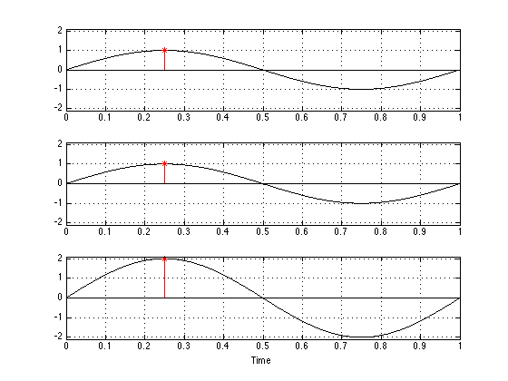
Remember we saw above in Fig.1 that, when you have two high pressure zones that meet each other, you get more pressure than either one of them alone. Now take a look at the animation above and look for the places where the black curves from the two “sources” intersect. This is where you’ll get an increase in pressure, and therefore more energy than just the direct sound by itself. As you can see in Fig. 3, below, this means that you have an angle off-axis to the front of the loudspeaker where the signal is louder than it is directly on-axis. Of course, this also means that there will be some angles where you hear less (because the secondary wavefront from the corner cancels the direct sound) – these are where the red and green curves (the high and low pressure zones) intersect.

 

 

As you can see in Fig 3a, there are different angles where the high pressures add to give you an even higher pressure (notice that the low pressures also add to give you an even lower pressure. The result is that, along those lines, you get constructive interference and therefore the sound is louder than it is elsewhere. I’ve only shown three such angles in this diagram – there are more. You might note as well that the origin of the high pressure lobes is not the centre of the loudspeaker driver (the piston shown in red). It’s somewhere between the primary and secondary sources (in this case, the loudspeaker driver and the corner).

 

 

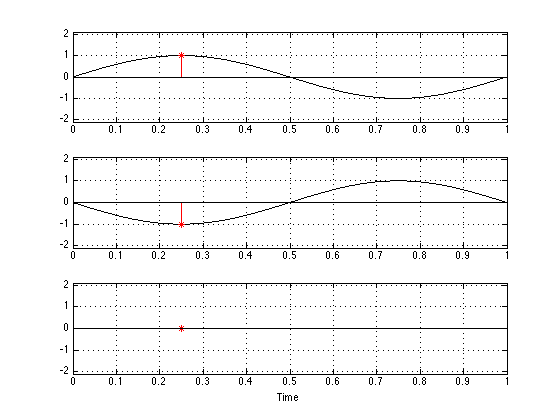
Fig 3b shows two angles where the high and the low pressures overlap, causing destructive interference and therefore cancellation. Therefore, the sound is quieter along those lines than it is elsewhere.

 

The real world

What does all of this mean in the real world?

Well, as you’ve probably already guessed, the first conclusion is that building a loudspeaker that has sharp corners is probably a bad idea. For example, if you wanted to build a loudspeaker, and you just put a tweeter on the front and made sharp right angles where the sides meet the front, you will have a problem with diffraction off those corners. As you can see in Figure 3, you will get a boost in the signal at some angles off-axis to the front of the loudspeaker, and some cancellation at other angles. The amount by which the signal will be boosted, the angles where you’ll have the effects, and the frequencies where you’ll have the problems are all dependent on the specific dimensions of the device. For example, the further away the loudspeaker’s corner from the driver, the lower the frequency that will be affected.

Let’s take a real-world example. The very first version prototype of the BeoLab 5 was really just a “normal” three-way loudspeaker that was used to test the ABC algorithm, So, there was a woofer in a cabinet with a microphone for the ABC development, but on top was just a small cabinet with a midrange driver and a tweeter, as you can see in Figures 4 and 5.

 

 

 

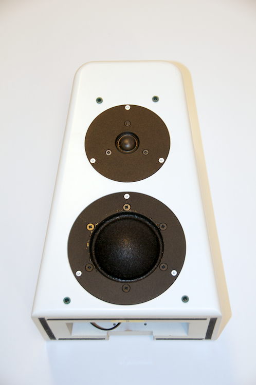
Figure 6 shows the “conventional” tweeter cabinet version of one of the BeoLab 5 prototypes which was placed on top of the white woofer cabinet shown in Figure 4 when the Acoustic Lens assembly was removed. As you can see, this is an example of how-not-to-make-a-loudspeaker (if you’re worried about diffraction). We have a tweeter in a flat surface and (some sharp-ish corners at the sides of the loudspeaker face). The result of this is that we have exactly the same problem shown in Figure 3a and 3b, above. We can see this in the measurement of the horizontal directivity of the loudspeaker, shown in Figure 7, below.

It may be a little difficult to read this plot, so I’ll explain a little. The entire plot has been normalised to the on-axis magnitude response of the tweeter. In other words, the measurement doesn’t show the response of the tweeter – it shows how the response changes as you move around the loudspeaker in the horizontal plane.  The X-axis is the frequency of the signal in Hz, ranging from 1.8 kHz to 20 kHz. The Y-axis is the horizontal angle of radiation of the loudspeaker where 0° is directly on-axis, in front the tweeter. The lines in the plot can be thought of as a kind of topographical map with a difference of 0.5 dB per contour. So, if you think of a straight “ridge” in the plot along the 0° line in the middle, the plot generally falls off (in other words, the signal is quieter) as you move around to the side and back of the loudspeaker. You can see that, at the high frequencies, the lines are closer together which means that you lose more level at high frequencies than at low frequencies as you come around to the side of the loudspeaker. This is traditionally called loudspeaker “beaming”. The interesting thing to look at are the four red oval areas. The larger ones are centred around 3.2 kHz and ±40°. The smaller ones are up at about 7.5 kHz and  about ±15°. Because they’re in red, this means that they are louder than the on-axis response, so they are peaks in the topographical map. These peaks are the direct result of diffraction off the edge of the loudspeaker cabinet.  I count 4 red contour lines at the lower frequency peak, which means that we have a beam that is about 2 dB (remember, 0.5 dB per line * 4 lines) louder around 3 kHz at 40° off-axis to the loudspeaker.

This cabinet was built compare the directivity of a normal box-shaped loudspeaker to one with an Acoustic Lens. A close-up of the lens used for this comparison is shown below in Figure 8.

 

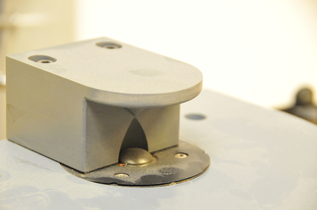
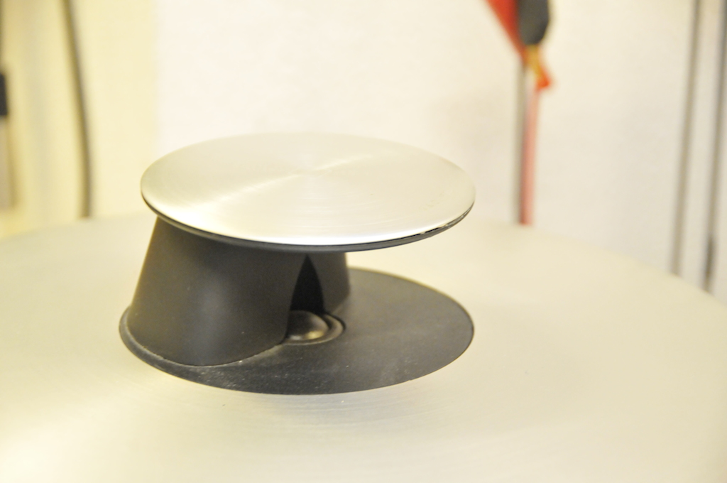
You’ll note in Figure 8 that the Acoustic Lens is slightly different from the final version (hence the “first-generation” qualifier) . This version also suffered from diffraction artefacts caused by the sharp edges where the face of the lens structure meets its side. This was corrected in the second generation version shown below in Figure 9.

 

Notice that the second-generation lens has curved transitions from face to side to reduce the diffraction problem. This curvature was eventually extended to wrap around the entire structure as can be seen in the photo of the final BeoLab 5 tweeter lens in Figure 10, below.

 

 

 

You may notice that the difference in these two designs was that the original one had sharp corners on the sides. The diffraction effects of these corners were easily visible in the first directivity measurements of the Lens, so the second prototype with the curved transition from front to side was made to eliminate this problem. The directivity measurement of the prototype shown in Figure 9 is seen below in Figure 11.

You’ll see in Figure 11 that there are two significant differences between the directivity of a tweeter in the prototype Acoustic Lens and a conventional cabinet (shown in Figure 7). The first difference is that the beaming effect (seen as a convergence of the contour lines at the high frequencies in Figure 7) does not happen with the lens. The contour lines are much more parallel resulting in a behaviour known as “constant directivity”. This is a way of saying that the loudspeaker has a directivity that is the roughly the same throughout its entire frequency range (rather than beaming in the high end).

The second difference is that the peaks in the 3 kHz and 8 kHz areas, seen in Figure 7, are gone. This is because there are no corners at the edge of the loudspeaker cabinet to cause diffraction. You may note a peak in the magnitude responses off-axis above 15 kHz. We actually don’t know what causes this, however, since it is so high in frequency and only +1 to +1.5 dB, and since this is still only a prototype, it wasn’t really considered to be a significant issue.

 

Wrapping up 

So, I’ve killed two birds with one stone in this article (or “two flies with one smack” as they say in Denmark). On the one hand,  we’ve seen that, if you’re worried about the directivity and/or the off-axis response of your loudspeaker (I know, the latter is a sub-set of the former…) sticking a tweeter (or a midrange, or a woofer, depending on dimensions and frequency ranges) on the front of a rectangular box is probably a really bad idea. (On the other hand, it’s a pretty easy, and therefore cheap, way to build a speaker, which is why such a design is so popular I guess…) And, on the other hand, we’ve seen one of the characteristics of Acoustic Lenses – being a more constant directivity than a tweeter-on-a-box. The fact that the tweeter mounted in an Acoustic Lens had less diffraction is not because of the Lens geometry in particular, but because of the shaping of its surroundings as part of the development process of BeoLab 5.

There are more stories like this one. For example, if you look carefully at the “plates” of the BeoLab 5 and the prototype in Figure 4 (the part the tweeter and midrange drivers are mounted in), you might notice that the prototype plates are flat, whereas the BeoLab 5 plates curve downwards. This is not because someone thought the curve would look pretty. This was because the circular edge of the prototype plates also caused diffraction, resulting in a higher-level lobe in the vertical plane. Sloping the plates downwards puts their sharp edges in the “shadow” of the plates themselves, reducing the diffraction effects. So, you can see that diffraction and its effects on directivity is one of the other issues that we worry about when we’re building a loudspeaker.