Rocks, Guitars, and Children
If you throw a rock into a pond on a windless day, you’ll see the ripples moving away in an expanding circle from the place where the rock hit. The ripples are places on the water where the water is either higher or lower than where it was before you hit the rock. The water itself only moves up and down, but the waves expand sideways. (You can see this if there is something floating on the water, for example – it bobs up and down as the waves go by.)
A similar thing happens when you pluck a guitar string. The point where your finger plucked is the same as the point where the rock landed in the water, and waves radiate away from that place on the string in two directions (because there are only two directions to travel in on a string: this way and that way). However, when those waves reach the end of the string, they reflect and come back in the opposite direction.
In both cases, the water and the guitar string, the wave has some speed at which it travels. It’s slow enough on the water for you to watch it, but it’s much too fast on a guitar string. In fact, it’s so fast that, when you pluck it, the wave travels to the end of the string, reflects in the opposite direction, hits the other end of the string, reflects again, and gets back to where you plucked it in about 1/82nd of a second if it’s the low E string. Since the wave doesn’t stop there – it keeps going, repeating the back-and-forth journey along the length of the string every 1/82nd of a second, then we hear a note with a fundamental frequency of 82 Hz (82 cycles per second): a low E.
That ringing that happens on the guitar string will happen no matter how you start the movement on it. You could hit the string with a chopstick, you could just thump the side of the guitar with your fist, you could even stand next to the guitar and cough loudly. All of these things will “inject” energy into the string, causing it to move, and the wave starts banging back and forth.
The rate of repetition is dependent on two things: the length of the string and the speed of the wave. The speed of the wave is dependent on two things: the mass of the string (e.g. how heavy is 1 m of it?) and the tension (how tightly is it stretched?) Increase the tension, and you increase the speed of the wave. Decrease the mass and you increase the speed of the wave. Increase the speed of the wave, and the repetition takes less time, so you hear a higher note.
That frequency at which the string will naturally ring is called a resonance. A child on a swing will go back and forth at the same rate (number of times per second) no matter how gently or forcefully you push them – apply energy, and the system will resonate.
Now, let’s think about that push of the child, the rock hitting the water, or the pluck of the guitar string. All of those things are a short injection of energy: a kind of impulse, and the way the child, the water, or the string behaves afterwards is its impulse response – how it responds to that impulse.
But here’s a strange thing to consider. This means that the note (the frequency) that you hear from the guitar string was one of the many frequencies in the initial pluck itself.
So, another way to think of this is that, by plucking the string, you inject a signal with all frequencies in it, and all of those frequencies decay (“die away”) very quickly except for one.
Okay, okay, if we’re going to be pedantic, I should be including not only the fundamental frequency but all of the additional harmonics; typically multiples of that frequency. But we don’t need to complicate things with the truth at the moment…
What does this have to do with filters?
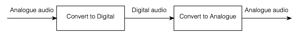
From a “big picture” point of view, a guitar string is a filter. I feed in some signal (the pluck) and I get out a modified version of that signal (the note ringing). From the same perspective, a filter in an equaliser is the same: I feed in a signal (music) and I get out a modified version of it (the same music, but slightly louder at 1 kHz, for example). What’s interesting is that the two things basically work the same way.
Let’s take the example of the filter at the end of Part 1: a peaking filter with a boost of 12 dB at 1 kHz, with a Q of 2. If I feed in a sine wave (which only contains energy at 1 frequency) at a very low frequency (say, 100 Hz or lower) then the level of the output will equal that of the input. If I do the same with a very high frequency (say, 10 kHz) then the level of the output will also equal that of the input. However, if I feed in a sine wave at 1 kHz, the output will be 4 times louder than the input (+12 dB = 4 time the amplitude because 20*log10(4) = 12-ish).
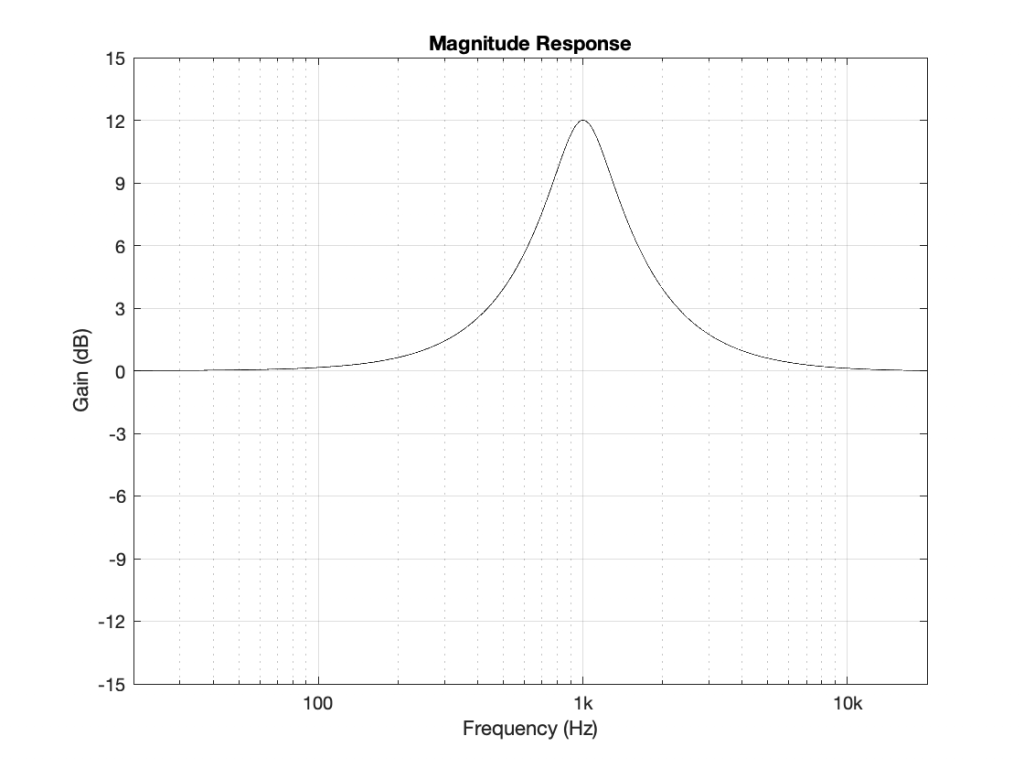
At some other frequency around 1 kHz, I’ll get a different answer. However, this is a VERY long and tedious way to measure the magnitude response of the filter. Another option is to measure its impulse response.
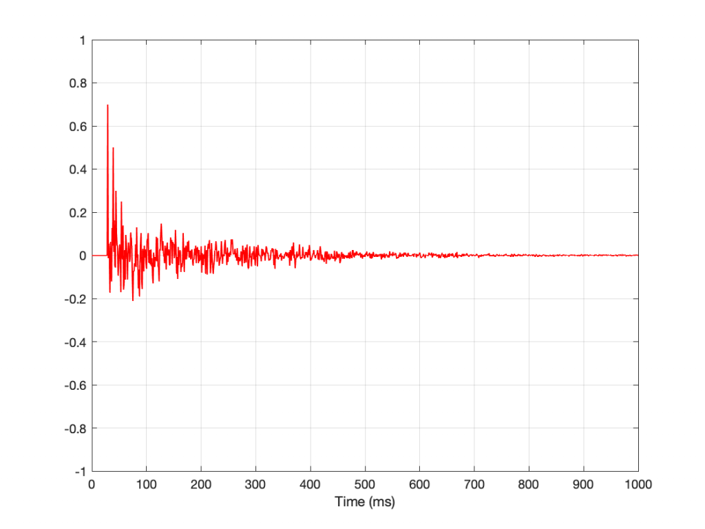
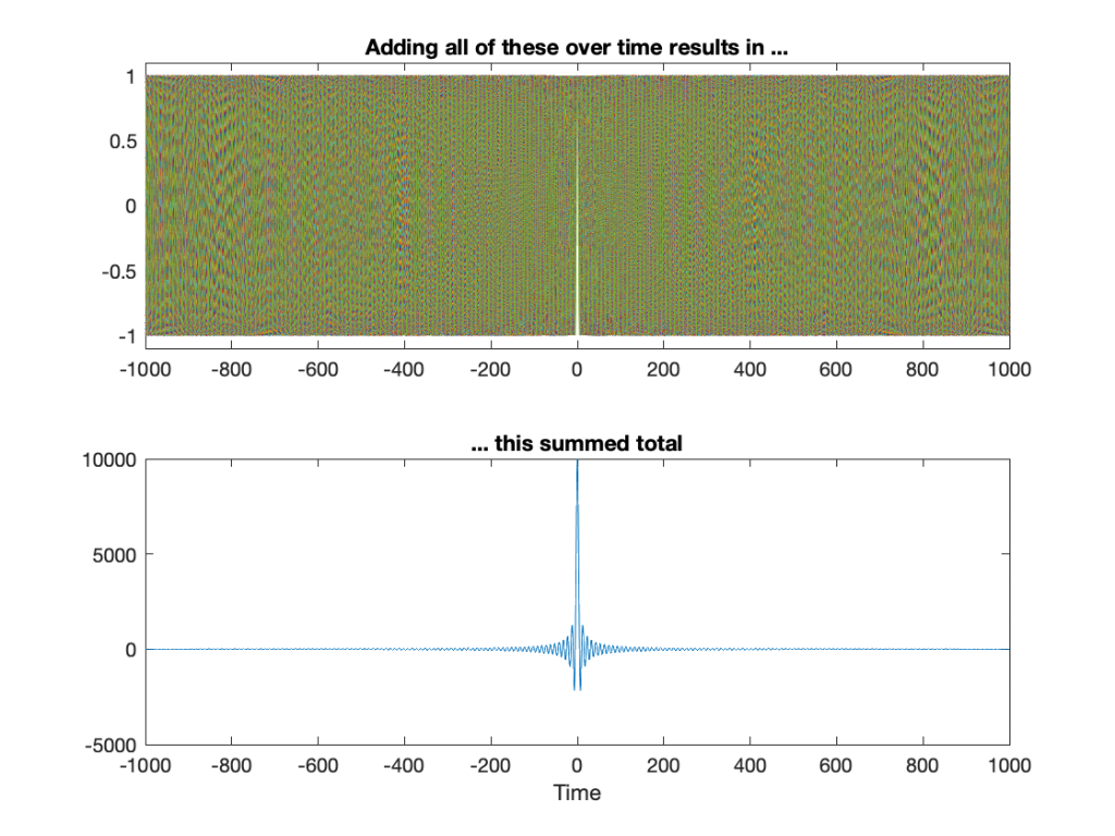
If I feed the input of the filter with an impulse (which is a sound that contains all frequencies at the same level, as we saw in Part 1), and look at the filters output in time, it might look like this:

Notice that the impulse looks like an impulse at Time = 0, but then something extra happens afterwards – like a guitar string ringing in time. If I zoom in vertically and look at the same plot, it will look like Figure 3.

And if we zoom in horizontally as well, it will look like this.
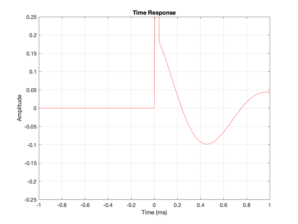
So, as you can see there, it’s almost as if we kept the impulse, and then just added a cosine wave with a period (a repetition time) of 1 ms, starting at Time = 0 and decaying over time. In fact, that’s exactly what the filter does.
Time response to Frequency response
The excuse I gave above for sending an impulse through the filter (instead of sine waves) was that this will be a faster way to measure its response. The time response of the filter is already done. We can see that in the figures above. But how do we see the filter’s frequency response? This is done using a clever bit of math called a Fourier Transform, which lets you take a signal in time, and analyse its content by frequency. I won’t explain that here, but if you’re interested in how it works, you can start by reading this.
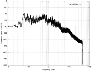
If I take the total impulse response (also known as a time response measurement) of the filter: in other words, I send in an impulse, I record the output and don’t stop recording until the ringing has decayed to a level low enough that I no longer care (for the purposes of this discussion, at least). Then, I do a Fourier Transform of the recording, I get something like Figure 5.
There is no new information in Figure 5. It’s just a setup for Figures 6 and 7.
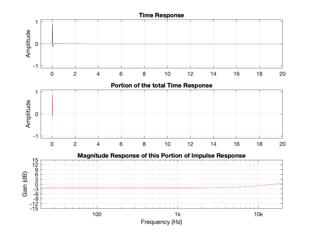
Let’s now start slicing up the time response selectively to see what frequencies are contained in the output of the filter at what time. We’ll start by just taking the first and second samples of the impulse at the output, shown in Figure 6.
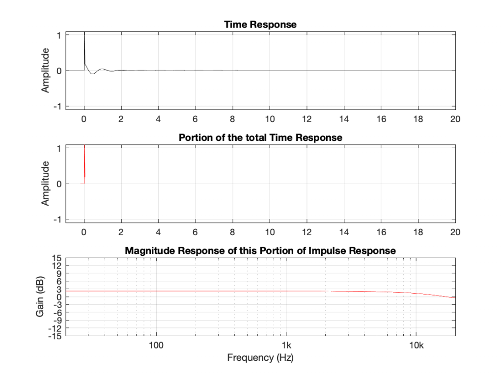
As you can see in Figure 6, if I remove the ringing that comes after the impulse, then the response of the signal has an almost-flat magnitude response and a gain of about 2 dB or so. This should not come as a surprise, since it’s almost an impulse. The only real difference between the portion that I’ve used and a real impulse is that the second value is not 0. So far so good…
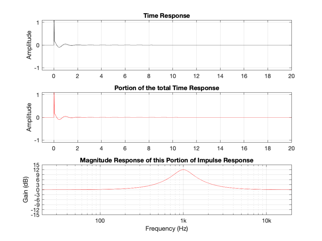
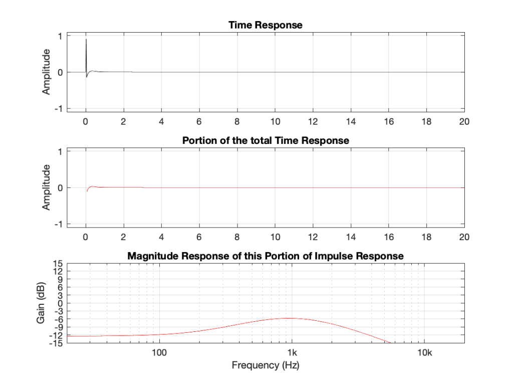
Let’s look at the remainder of the time response. This is shown in Figure 7.
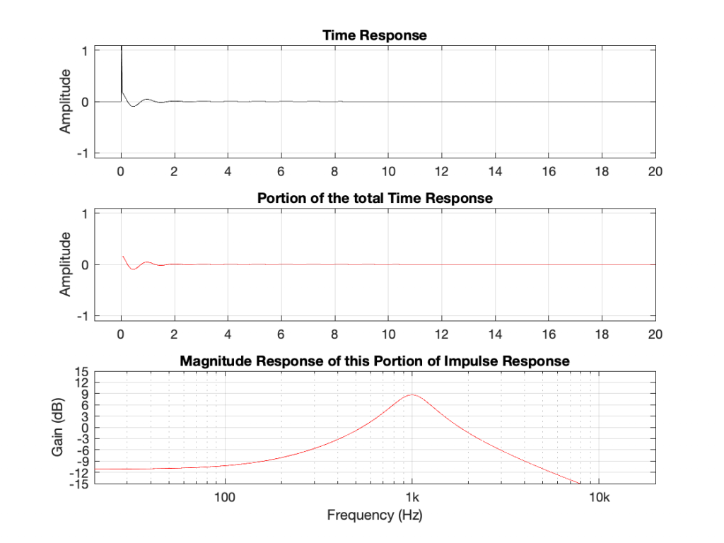
Figure 7 shows something interesting. We see the response of a band-pass filter with a centre frequency of 1 kHz, and a gain of 9 dB, which is the response of the filter after the initial impulse has passed.
What does this all mean!?
If we leave out one important thing for now, this means that a peaking filter that has a boost of 12 dB, an Fc of 1 kHz and a Q of 2 is actually the sum of two things:
- a through-put with a little gain (about 1 dB)
- a bandpass filter with a gain of about 9 dB
This is, in essence, true. You can create a peaking filter by summing a bandpass filter to a through-put. However, an important point to realise here is that the band pass signal essentially comes after the onset of the signal. In Part 3, we’ll talk about whether this is a problem – or, more accurately, when this might be a problem. For now, however, I’ll throw one more example at you.
Up to now, we’ve only looked at the example of a peaking filter with a boost. What happens when the filter has a cut instead?
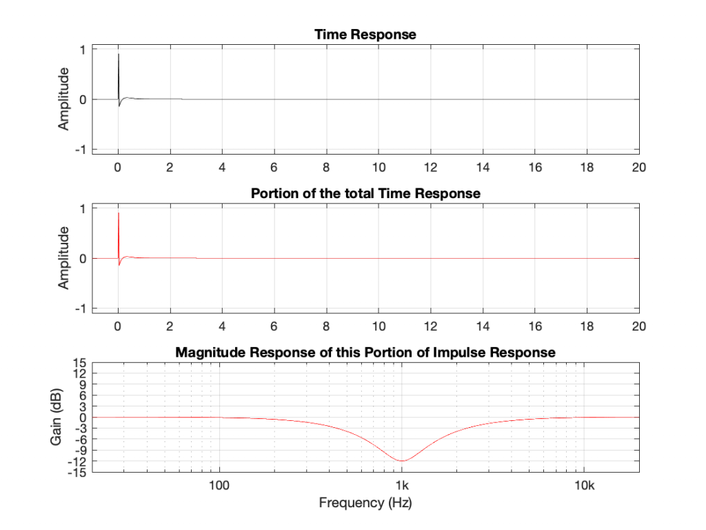
Notice that a dip filter also rings in time after the initial impulse, but decays much faster than the equivalent boost. (I’ll have to be a bit more careful about my use of the word “equivalent”, actually – but I’ll straighten that out at the end of the series. To be continued…)
Okay, what’s going on here? A peaking filter with a boost is a through-put plus a bandpass. A dip filter is ALSO a through-put plus a somewhat quieter (sort-of) bandpass. This doesn’t make any sense.
Actually it doesn’t make any sense because there’s a piece of information that I’m leaving out – the phase of the ringing. Notice that, with the peaking filter, the decay portion starts positive and then goes negative initially. With the dip filter, the decay starts negative and goes positive. So, the previous paragraph should have read: “A peaking filter with a boost is a through-put PLUS a bandpass. A dip filter is ALSO a through-put MINUS a somewhat quieter (sort-of) bandpass.”
The phases of the decays of the bandpass portions are opposite for the two filters. Another way to think of this is that the ringing in the dip filter cancels the energy around 1 kHz in the initial impulse, whereas the ringing in the peak filter adds to it.
However, it’s really important to note for now that both filters – the peak and the dip result in ringing in time.