After I posted the last two parts of this series (which I thought wrapped it up…) I received an email asking about whether there’s a similar thing happening if you remove the reconstruction (low-pass) filter in the digital-to-analogue part of the signal path.
The answer to this question turned out to be more interesting than I expected… So I wound up turning it into a “Part 3” in the series.
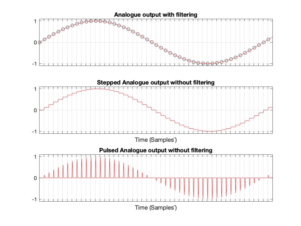
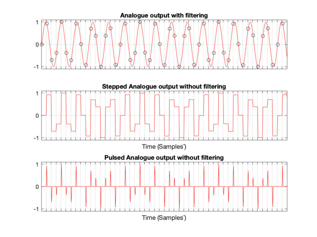
Let’s take a case where you have a 1 kHz signal in a 48 kHz system. The figure below shows three plots. The top plot shows the individual sample values as black circles on a red line, which is the analogue output of a DAC with a reconstruction filter.
The middle plot shows what the analogue output of the DAC would look like if we implemented a Sample-and-hold on the sample values, and we had an infinite analogue bandwidth (which means that the steps have instantaneous transitions and perfect right angles).
The bottom plot shows what the analogue output of the DAC would look like if we implemented the signal as a pulse wave instead, but if we still we had an infinite analogue bandwidth. (Well… sort of…. Those pulses aren’t infinitely short. But they’re short enough to continue with this story.)
Figure 1. A 1 kHz sine wave
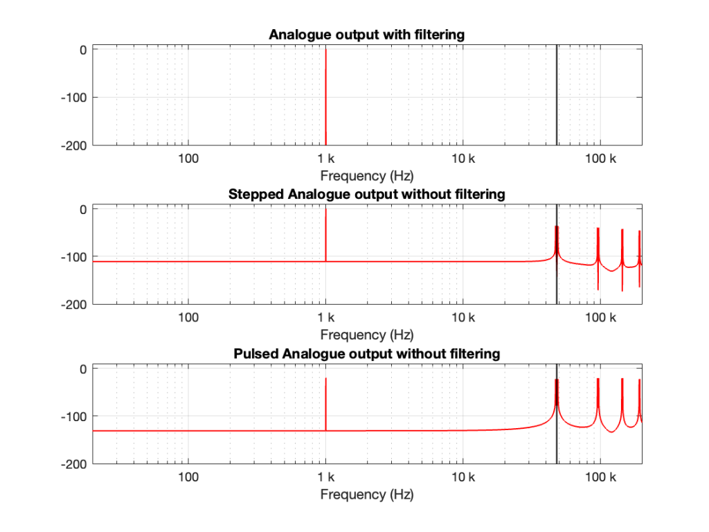
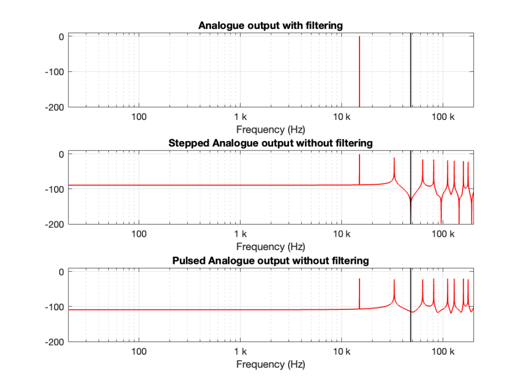
If we calculate the spectra of these three signals , they’ll look like the responses shown in Figure 2.
Figure 2. The spectra of the signals in Figure 1.
Notice that all three have a spike at 1 kHz, as we would expect. The outputs of the stepped wave and the pulsed wave have much higher “noise” floors, as well as artefacts in the high frequencies. I’ve indicated the sampling rate at 48 kHz as a vertical black line to make things easy to see.
We’ll come back to those artefacts below.
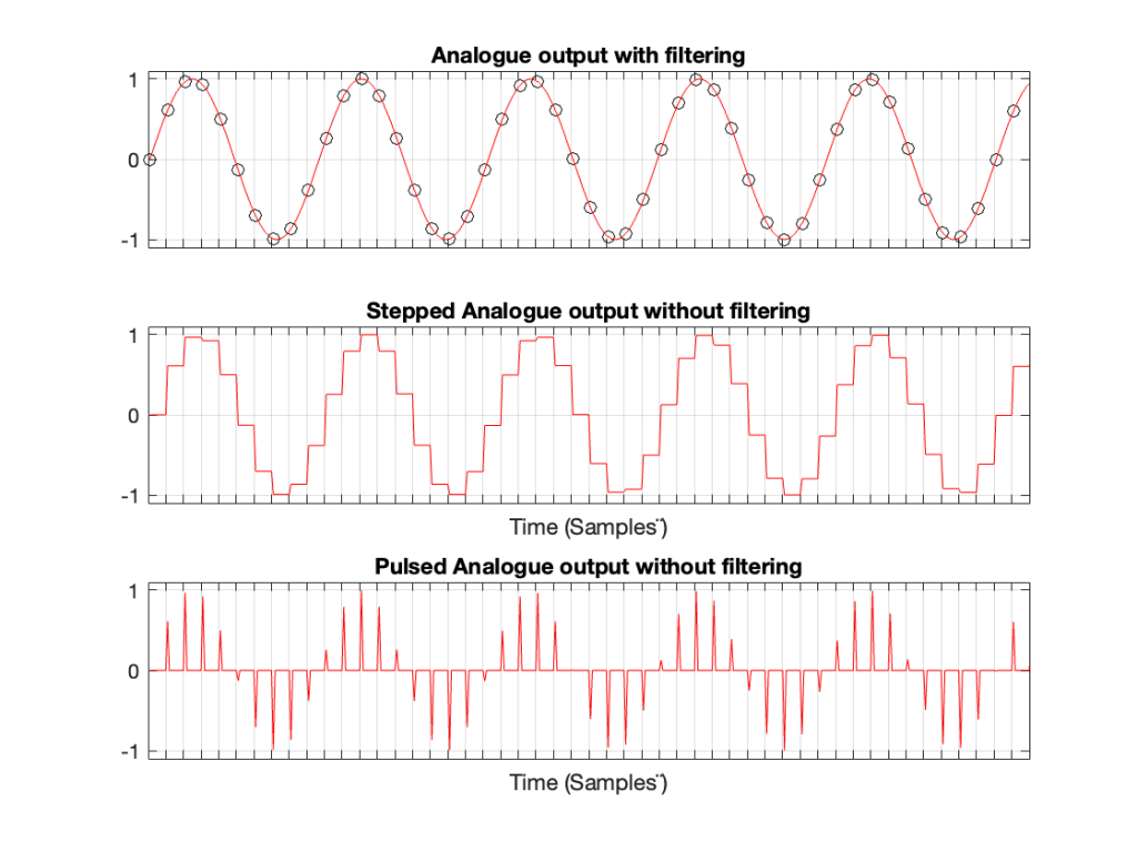
Let’s do the same thing for a 5 kHz sine wave, still in a 48 kHz system, seen in Figures 3 and 4.
Figure 3. A 5 kHz sine wave
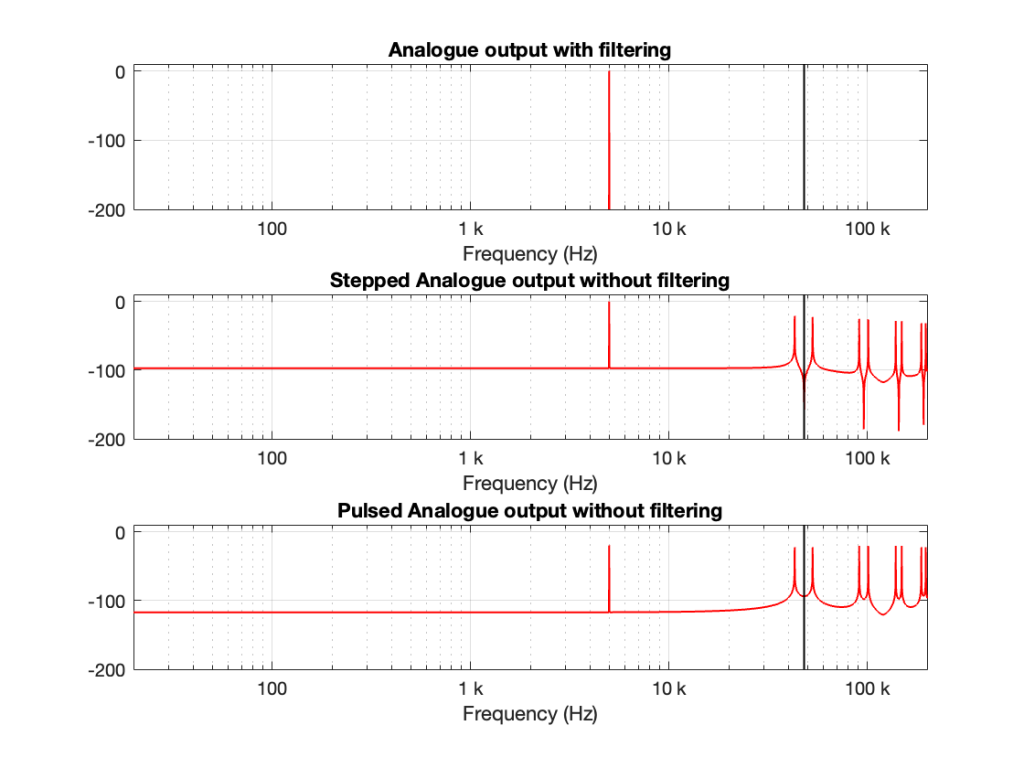
Figure 4. The spectra of the signals in Figure 3.
Compare the high-frequency artefacts in Figure 4 to those in Figure 2.
Now, we’ll do it again for a 15 kHz sine wave.
Figure 5. A 15 kHz sine wave
Figure 6. The spectra of the signals in Figure 5.
There are three things to notice, comparing Figures 2, 4, and 6.
The first thing is that artefacts for the stepped and pulsed waves have the same frequency components.
The second thing is that those artefacts are related to the signal frequency and the sampling rate. For example, the two spikes immediately adjacent to the sampling rate are Fs ± Fc where Fs is the sampling rate and Fc is the frequency of the sine wave. The higher-frequency artefacts are mirrors around multiples of the sampling rate. So, we can generalise to say that the artefacts will appear at
n * Fs ± Fc
where n is an integer value.
This is interesting because it’s aliasing, but it’s aliasing around the sampling rate instead of the Nyquist Frequency, which is what happens at the ADC and inside the digital domain before the DAC.
The third thing is a minor issue. This is the fact that the level of the fundamental frequency in the pulsed wave is lower than it is for the stepped wave. This should not be a surprise, since there’s inherently less energy in that wave (since, most of the time, it’s sitting at 0). However, the artefacts have roughly the same levels; the higher-frequency ones have even higher levels than in the case of the stepped wave. So, the “signal to THD+N” of the pulsed wave is lower than for the stepped wave.
One of the best-known things about digital audio is the fact that you cannot record a signal that has a frequency that is higher than 1/2 the sampling rate.
Now, to be fair, that statement is not true. You CAN record a signal that has a frequency that is higher than 1/2 the sampling rate. You just won’t be able to play it back properly, because what comes out of the playback will not be the original frequency, but an alias of it.
If you record a one-spoked wheel with a series of photographs (in the old days, we called this ‘a movie’), the photos (the frames of the movie) might look something like this:
As you can see there, the wheel happens to be turning at a speed that results in it rotating 45º every frame.
The equivalent of this in a digital audio world would be if we were recording a sine wave that rotated (yes…. rotated…) 45º every sample, like this:
Notice that the red lines indicating the sample values are equivalent to the height of the spoke at the wheel rim in the first figure.
If we speed up the wheel’s rotation so that it rotated 90º per frame, it looks like this:
And the audio equivalent would look like this:
Speeding up even more to 135º per frame, we get this:
and this:
Then we get to a magical speed where the wheel rotated 180º per frame. At this speed, it appears when we look at the playback of the film that the wheel has stopped, and it now has two spokes.
In the audio equivalent, it looks like the result is that we have no output, as shown below.
However, this isn’t really true. It’s just an artefact of the fact that I chose to plot a sine wave. If I were to change the phase of this to be a cosine wave (at the same frequency) instead, for example, then it would definitely have an output.
At this point, the frequency of the audio signal is 1/2 the sampling rate.
What happens if the wheel goes even faster (and audio signal’s frequency goes above this)?
Notice that the wheel is now making more than a half-turn per frame. We can still record it. However, when we play it back, it doesn’t look like what happened. It looks like the wheel is going backwards like this:
Similarly, if we record a sine wave that has a frequency that is higher than 1/2 the sampling rate like this:
Then, when we play it back, we get a lower frequency that fits the samples, like this:
Just a little math
There is a simple way to calculate the frequency of the signal that you get out of the system if you know the sampling rate and the frequency of the signal that you tried to record.
Let’s use the following abbreviations to make it easy to state:
Fs = Sampling rate
F_in = frequency of the input signal
F_out = frequency of the output signal
IF F_in < Fs/2 THEN F_out = F_in
IF Fs > F_in > Fs/2 THEN F_out = Fs/2 – (F_in – Fs/2) = Fs – F_in
Some examples:
If your sampling rate is 48 kHz, and you try to record a 25 kHz sine wave, then the signal that you will play back will be: 48000 – 25000 = 23000 Hz
If your sampling rate is 48 kHz, and you try to record a 42 kHz sine wave, then the signal that you will play back will be: 48000 – 42000 = 6000 Hz
So, as you can see there, as the input signal’s frequency goes up, the alias frequency of the signal (the one you hear at the output) will go down.
There’s one more thing…
Go back and look at that last figure showing the playback signal of the sine wave. It looks like the sine wave has an inverted polarity compared to the signal that came into the system (notice that it starts on a downwards-slope whereas the input signal started on an upwards-slope). However, the polarity of the sine wave is NOT inverted. Nor has the phase shifted. The sine wave that you’re hearing at the output is going backwards in time compared to the signal at the input, just like the wheel appears to be rotating backwards when it’s actually going forwards.
In Part 2, we’ll talk about why you don’t need to worry about this in the real world, except when you REALLY need to worry about it.
Back when I was at McGill, one of my fellow Ph.D. students was Mark Ballora, who did his doctorate in converting heart rate data to an audible signal that helped doctors to easily diagnose patients suffering from sleep apnea.
As I’ve stated a couple of times through this series, my reason for writing this stuff was not to prove that high res audio is better or worse than normal res audio (whatever that is…). My reason was to highlight some of the advantages and disadvantages associated with LPCM audio at different bit depths and sampling rates. Just as a bullet-point summary of things-to-remember/consider (with some loose grouping):
“High resolution audio” could mean
“more than 16 bits per sample” or
“a sampling rate higher than 44.1 kHz” or
both.
These two dimensions of the specifications have different implications on the signal
Just because you have more bits per sample doesn’t mean that you are actually getting more resolution. There are examples out there where a “24-bit recording” is just a 16-bit recording with 8 zeros stuck on the end.
Just because you have a higher sampling rate doesn’t mean that you are actually getting a recording that was done at that sampling rate. There are examples out there where, if you do a spectral analysis of a “high-res” recording, you’ll see the cutoff filter of the original 44.1 kHz recording.
Just because you have a recording done at a higher sampling rate doesn’t mean that the extra information you get is actually useful.
If your processing distorts the signal for some reason, it’s better to have a higher sampling rate to keep the aliased distortion artefacts as far away from the audio signal as possible.
If you are a lazy DSP engineer who thinks that filters give you the expected magnitude response, no matter what the centre frequency, you’d better have a higher sampling rate. (Or you could just stop being lazy and compensate.)
If you need a lower noise floor for the same audio bandwidth, it’s more efficient to add bits than to increase the sampling rate.
If you have a volume control after the conversion to analogue, then 93 dB of dynamic range (16 bits, TPDF dithered) might be enough – especially if you listen to music with a limited dynamic range. However, if your volume control is in the digital domain, and you have a speaker that can play loudly, then you’ll probably want more dynamic range, and therefore more bits per sample hitting the DAC.
Like I said, I’m not here to tell you that one thing is better or worse than another thing.
As I said, my intention in writing all of this is to help you to never fall into the trap of assuming that “high resolution audio” is better than “normal resolution audio” in all respects.
More is not necessarily better, sometimes, it’s not even more. Don’t fall victim to misleading advertising.
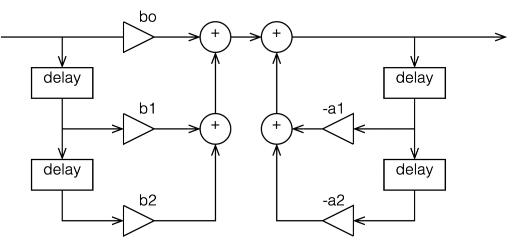
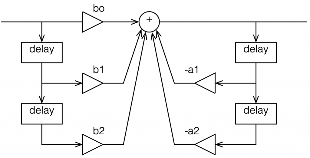
In the previous posting, we left off with this drawing of a biquad filter:
Figure 1: A biquad broken into an FIR filter with two 1-sample long delays and 3 gains combined with an IIR filter with two delays and 2 gains.
This is not the normal way to draw the signal flow inside a biquad, since it has a little too much information. Normally you see something like this:
Figure 2: A Biquad shown in “Direct Form 1” implementation with the feed forwards coming first.
or this:
Figure 3: A simpler way to show the same thing
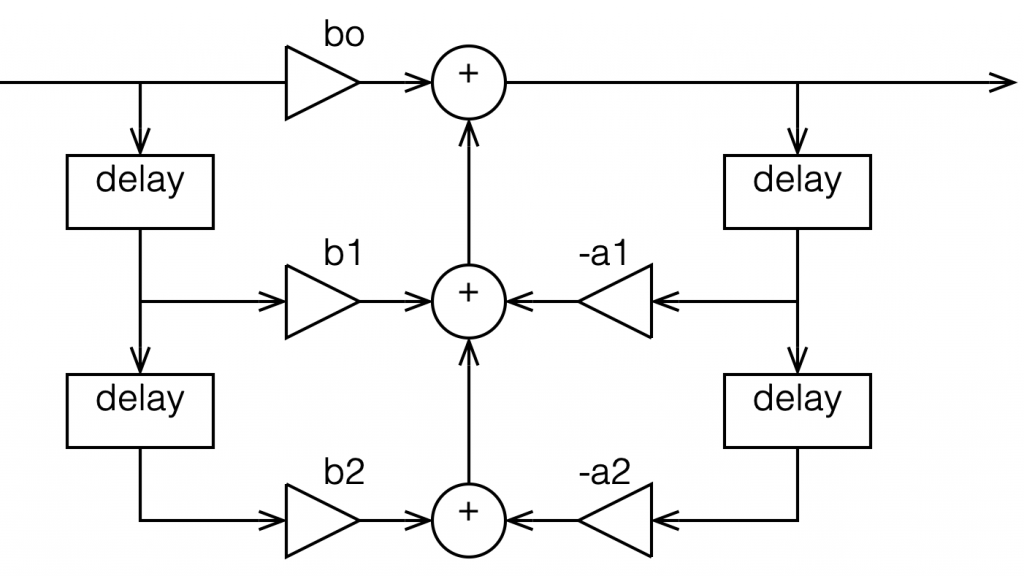
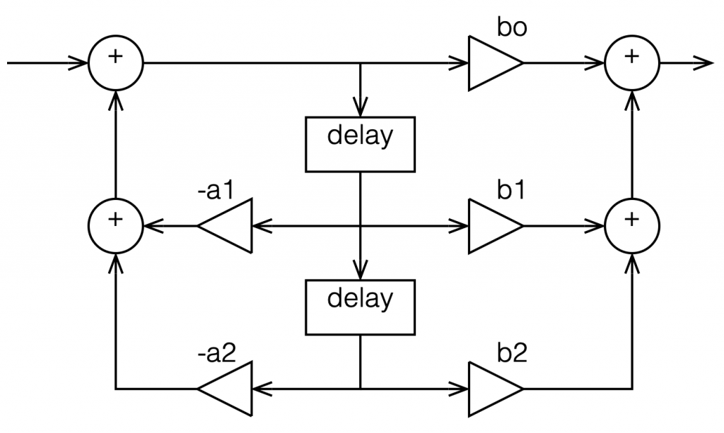
In the versions I show above, the feed-forward half of the biquad comes first, and its output feeds the start of the feedback portion. It is also possible to reverse these, putting the feedback portion first, like this:
Figure 4: A Biquad shown in “Direct Form 2” implementation with the feedback loops coming first.
In theory, these different implementations will all result in the same output if you match the gain values. However, in practice, they are not the same, and this difference is where we need to look for this part of the discussion on high res audio.
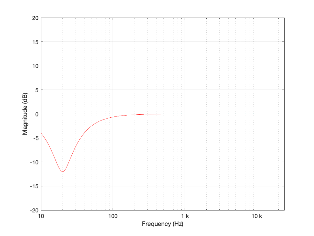
Let’s say I want to make a simple filter that reduces bass in a fairly narrow frequency band. I can use a biquad to do this. For example, if I want a peaking filter that reduces 20 Hz by 12 dB, with a Q of 1, then I get a magnitude response that looks like this:
Figure 5: The magnitude response of a peaking filter where F = 20 Hz, G = -12 dB, Q = 1
If I wanted to build this filter using a biquad in a system with a sampling rate of 48 kHz, it would have the following gain coefficients:
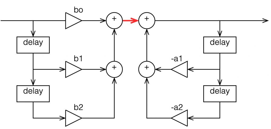
We’ll also say that my biquad is implemented like the one shown in Figure 1, above… let’s take a look at that signal flow again:
Figure 6: A copy of Figure 1 with one interior point in the signal flow highlighted in red.
I’ve highlighted a point inside the biquad using a red arrow. Let’s talk about the signal right there, in the middle of the processing…
In the last post, we talked about how, when the signal frequency is very low, a single sample delay has almost the same value at its output as its input, because the phase difference is so small for such a small time. So, let’s start with the (incorrect) assumption that, for those two feed-forward delays at the beginning, their outputs ARE equal to their inputs (because we’re starting with a low frequency). What happens when the input has a value of 1? Then the value at the red arrow is just the sum of the feed forward gains (because I multiplied each of them by 1 and added them together…)
In the case of the filter I described above, this value will be 0.000006836, which is a very small number. Also, if the value coming into the input of the biquad is less than 1, the value at the red arrow will be even smaller! This means that, if you come into the biquad with a low-frequency tone with a level of 0 dB FS, the level at that red arrow will be about -103 dB FS, which is very quiet. The feed-back portion of the biquad, after the red arrow, then has a lot of gain in it to bring the signal level back up towards 0 dB FS again.
So, the issue that we have here is that the FF (Feed Forward) portion of the biquad drops the level A LOT. And the FB portion increases the level A LOT, just to do something like a little 12 dB dip at 20 Hz.
The magnitude of the gains downwards and upwards in those two portions of the biquad are dependent on the parameters of the filter that we’re trying to make, however, we can generalise a little and say that:
the lower the frequency OR
the higher the Q,
then the bigger the gain down and up.
In other words, if you have a really low frequency dip, with a really high Q, then the level of the signal at that red arrow will be really low. REALLY low.
How low can you go?
How low is “REALLY low”? let’s see:
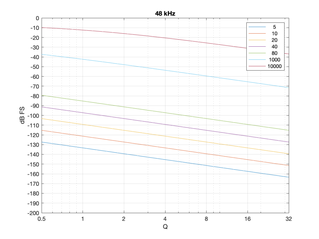
Figure 7: The level of a 0 dB FS signal at various frequencies listed in the top right corner, measured inside the biquad shown in Figure 6 at the red arrow, for a peaking filter with a gain of -12 dB, and with variable Q and Fc, in a system running at 48 kHz.
Take a look at Figure 7, which shows some values for one example filter (peaking, Gain = -12 dB, variable Q and Fc, and the test frequency = Fc). Notice that when the Fc is 10 kHz, even at earn Q=32, the signal level at the middle of the biquad is about -38 dB FS or so. However, when the Fc is 20 Hz, it’s -140 dB FS… This is very low.
Now let’s try again at a higher sampling rate: 192 kHz.
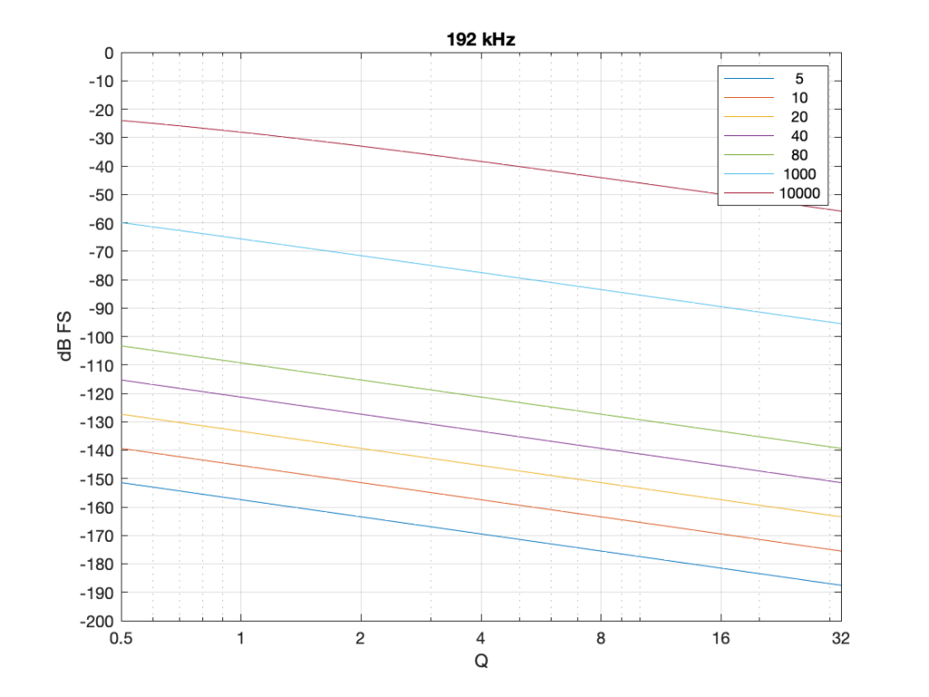
Figure 8: Identical parameters to that shown in Figure 7, but in a system running at 192 kHz.
Notice that when we do exactly the same thing running at 192 kHz, the signal levels inside the biquad get much lower. Now for a 20 Hz signal and a Q of 32, the level is around -163 dB FS – a drop of more than 20 dB for 4x the sampling rate.
Why does this happen? It’s because the filter doesn’t “know” that the signal is at 20 Hz. It only knows the relationship between the frequency and the sampling rate. So, in its little world, 20 Hz doesn’t exist. In a system running at 48 kHz, what exists is 20 / 48000 = 0.0004167. This is called the “normalised frequency” where the sampling rate is 1, DC is 0, and everything else is in between. (Note that some textbooks and software say that Nyquist = 1 instead of the sampling rate – but you just need to know what the convention is for the thing you’re reading…) This means that if the sampling rate goes up to 192 kHz, then the normalised frequency for 20 Hz is 20 / 192000 = 0.0001042 (1/4 of the value because the sampling rate was multiplied by 4).
So what?
This is important. If you want to make a low-frequency, high-Q peaking filter in a digital system with a cut of 12 dB, you are forcing the signal to a very low level inside your filter, and then bringing it back up to a normal level again on the way out. If your processing is running with a limited resolution, (e.g. 16-bits, for example) then the signal level can approach or even go below the resolution of your system inside the biquad. This means that, when the signal’s level is raised again on the way out, it’s full of quantisation distortion, and you can’t get rid of it… This is bad.
There are different ways to solve this problem.
Increase the resolution of your processing internally. For example, even though your input and output might only be running at 16-bits or 24-bits, maybe you need more resolution inside to make the results of the math better – or at least below the limitations of the input and output.
Change the way the biquad is implemented. For example, if you use the implementation shown in Figure 4 (with the feedback before the feed-forward) instead of the one we used, then you don’t drop the signal level and raise it again, you do the opposite. This avoids your quantisation error problem. However, depending on the system, it might overload and clip the signal inside the biquad instead, so then you just end up with a different kind of distortion instead.
Reduce your sampling rate to make it closer to your filter’s frequency. The problem I showed above is that the centre frequency of the filter is too far away from the sampling rate. If the sampling rate were lower, then this automatically makes the filter’s centre frequency “higher” in a normalised frequency scale, thus reducing the problem.
Other, even more clever solutions that I won’t talk about because they’re not as simple.
This means (for example) that if you’re building a subwoofer with digital filtering, and you know for sure that NOTHING will come out of it above, say 1 kHz (just to pick a random number that’s far enough away from the typical 120 Hz that people normally use…) then it would be dumb to do the filtering at 192 kHz. It’s smarter to run its internal sampling rate at 2 kHz (because we only need to go up to 1 kHz; and we’re not considering anything other issues or artefacts in this posting.)
P.S.
For this discussion, I used the specific example of a peaking filter with a gain of -12 dB, and I was varying the Q and the Fc. I was also measuring the level of the signal using a sine wave with a frequency that was the same as Fc in each case. However, the general lesson here about low frequency and high-Q filtering holds for other filter types and implementations as well.
I spent some time this week helping to track down the source of an error in a digital audio signal flow chain, and we wound up having a discussion that I thought might be worth repeating here.
Let’s start at the very beginning.
Let’s take an analogue audio signal and convert it to a Linear Pulse Code Modulation (LPCM) representation in the dumbest possible way.
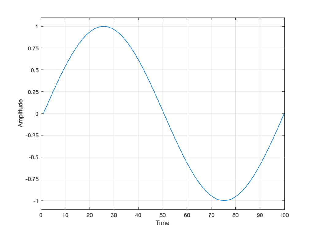
Fig 1. A simple analogue signal that we’ll use for the purposes of this discussion.
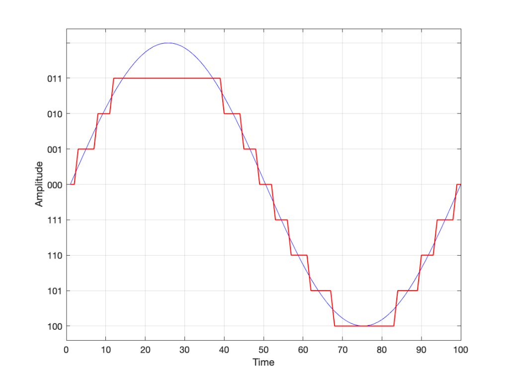
In order to save this signal as a string of numerical values, we have to first accept the fact that we don’t have an infinite number of numbers to use. So, we have to round off the signal to the nearest usable value or “quantisation value”. This process of rounding the value is called “quantisation”.
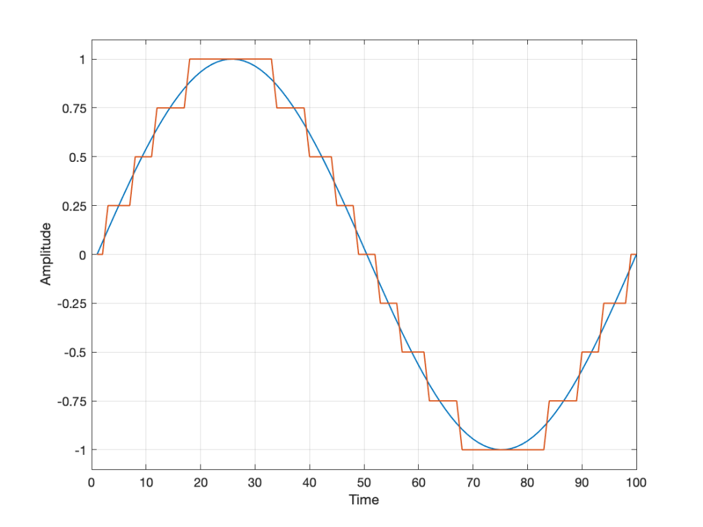
Let’s say for now that our available quantisation values are the ones shown on the grid. If we then take our original sine wave and round it to those values, we get the result shown below.
Fig 2. The original signal is shown as the blue line. The quantized version of it is shown as the red line.
Of course, I’m leaving out a lot of important details here like anti-aliasing filtering and dither (I said that we were going to be dumb…) but those things don’t matter for this discussion.
So far so good. However, we have to be a bit more specific: an LPCM system encodes the values using binary representations of the values. So, a quantisation value of “0.25”, as shown above isn’t helpful. So, let’s make a “baby” LPCM system with only 3 bits (meaning that we have three Binary digITs available to represent our values).
To start, let’s count using a 3-bit system:
Binary Value
4s place
2s place
1s place
Decimal Value
000
=
0 x 4 +
0 x 2 +
0 x 1
=
0
001
=
0 x 4 +
0 x 2 +
1 x 1
=
1
010
=
0 x 4 +
1 x 2 +
0 x 1
=
2
011
=
0 x 4 +
1 x 2 +
1 x 1
=
3
100
=
1 x 4 +
0 x 2 +
0 x 1
=
4
101
=
1 x 4 +
0 x 2 +
1 x 1
=
5
110
=
1 x 4 +
1 x 2 +
0 x 1
=
6
111
=
1 x 4 +
1 x 2 +
1 x 1
=
7
Table 1: The 8 numbers that can be represented using a 3-bit binary representation
and that’s as far as we can go before needing 4 bits. However, for now, that’s enough.
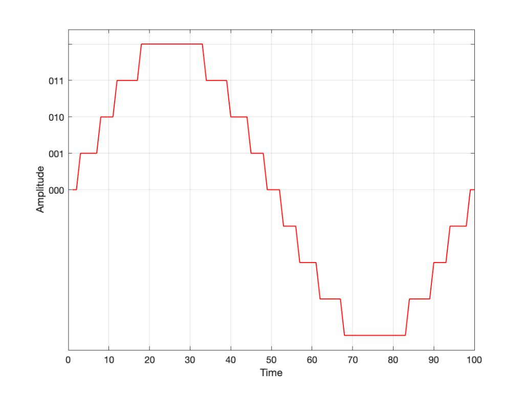
Take a look at our signal. It ranges from -1 to 1 and 0 is in the middle. So, if we say that the “0” in our original signal is encoded as “000” in our 3-bit system, then we just count upwards from there as follows:
Fig 3. Starting at 000 for the “0” value, and counting upwards into the positive values.
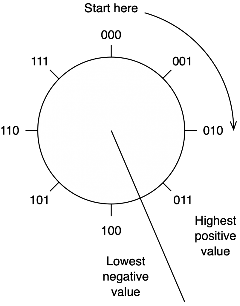
Now what? Well, let’s look at this a little differently. If we were to divide a circle into the same number of quantisation values, make the “12:00” position = 000, and count clockwise, it would look like this:
Fig 4. Counting from 000 to 111 around a circle
The question now is “how do we number the negative values?” but the answer is already in the circle shown above… If I make it a little more obvious, then the answer is shown below.
Fig 5. Relating the values on the circle to the values we’ll need to represent the audio signal…
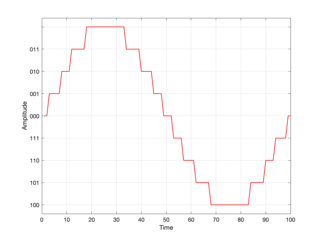
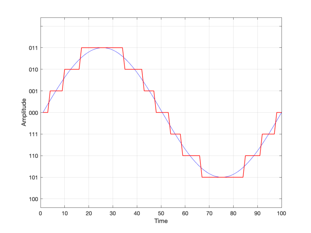
If we use the convention shown above, and represent that on the graph of our audio signal, then it looks like this:
Fig. 6
One nice thing about this way of doing things is that you just need to look at the first digit in the binary word to know whether the value is positive or negative. A 0 means it’s positive, and a 1 means it’s negative.
However, there are two issues here that we need to sort out… The first is that, since we have an even number of values, but an odd number of quantisation steps (4 above zero, 4 below zero, and zero = 9 steps) then we had to do something asymmetrical. As you can see in the plot above, there are no numbers assigned to the top quantisation value, which actually means that it doesn’t exist.
So, if we’re still being dumb, then the result of our quantisation will either look like this:
Fig 7. The dumb way to deal with the asymmetrical quantisation problem. Notice that the result is asymmetrically clipped on the positive side, but not the negative.
or this:
Fig 8. A smarter way to deal with the asymmetrical quantisation problem. Notice that we’ll never use the bottom value.
Wrapping up…
But what happens when you make two mistakes simultaneously? Let’s go back and look at an earlier plot.
Fig 9.
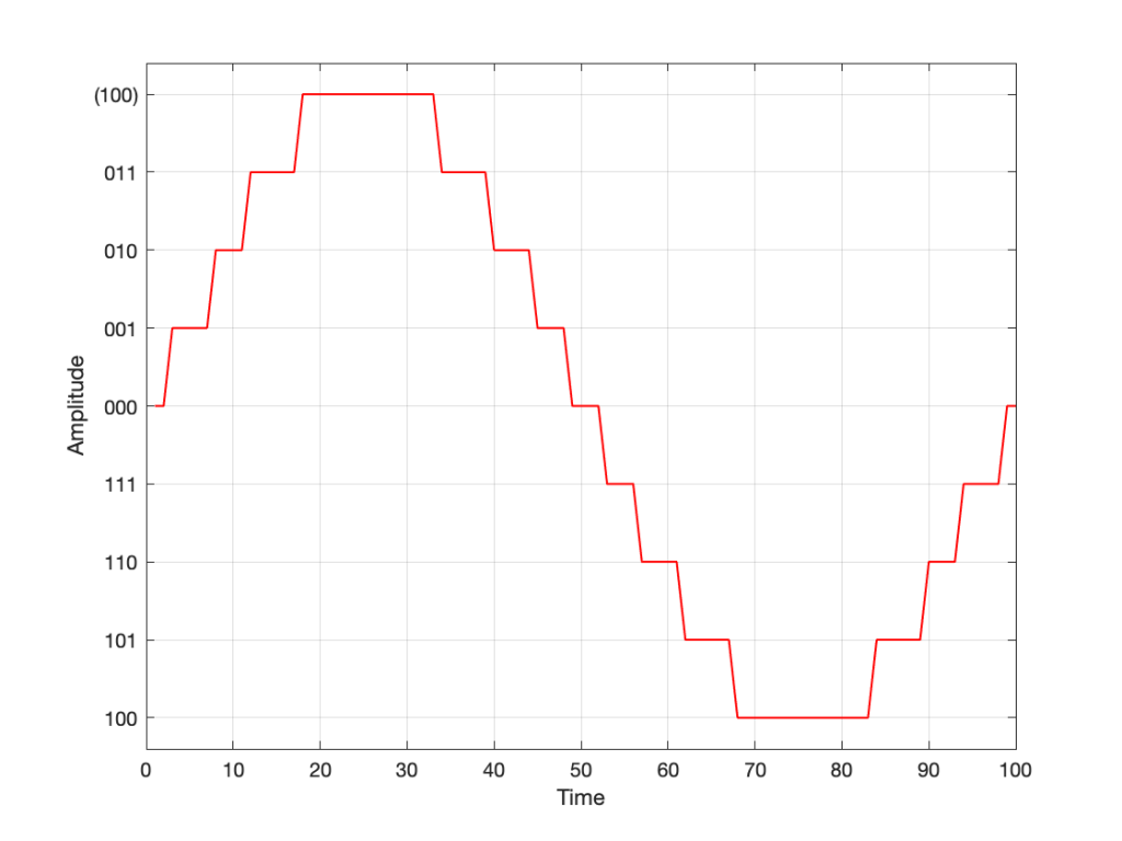
Let’s say that you’re writing some DSP code, and you forget about the asymmetry problem, so you scale things so they’ll TRY to look like the plot above.
However, as we already know, that top quantisation value doesn’t exist – but the code will try to put something there. If you’ve forgotten about this, then the system will THINK that you want this:
Fig 10. Notice that top quantisation value. I’ve labeled it as (100) because that’s the binary number after 011 – but 100 is ACTUALLY already used for the bottom-most negative value… Bad things are about to happen.
As you can see there, your code (because you’ve forgotten to write an IF-THEN statement) will think that the top-most positive quantisation value is just the number after 011, which is 100. However, that value means something totally different… So, the result coming out will ACTUALLY look like this:
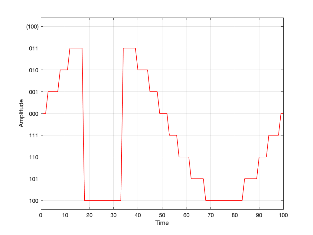
Fig 11. The actual output resulting from the mistakes described above.
As you can see there, the signal is very different from what we think it should be.
This error is called a “wrapping” error, because the signal is “wrapped” too far around the circle shown in Figure 5, shown above. It sounds very bad – much worse than “normal” clipping (as shown in Figure 7) because of that huge nearly-instantaneous transition from maximum positive to maximum negative and back.
Of course, the wrapping can also happen in the opposite direction; a negatively-clipped signal can wrap around and show up at the top of the positive values. The reason is the same because the values are trying to go around the same circle.
As I said: this is actually the result of two problems that both have to occur in the same system:
The signal has to be trying to get to a level that is beyond the limits of the quantisation values
Someone forgot to write a line of code that makes sure that, when that happens, the signal is “just” clipped and not wrapped.
So, if the second of these issues is sitting there, unresolved, but the signal never exceeds the limits, then you’ll never have a problem. However, I will never need the airbags in my car, unless I have an accident. So, it’s best to remember to look after that second issue… just in case.
P.S.
This method of encoding the quantisation values is called the “Two’s Complement” method. If you want to know more about it, read this.
There was an article in the BBC News webpage this week, telling the story of how Leon Theremin (inventor of one of the first electronic musical instruments) invented the technology underneath what we now call RFID…
Of course, this means that every time I swipe my card to buy something at the store, I’m going to start humming the hook from”Good Vibrations”… Maybe knowledge is not always a good thing… Or maybe I should get out my Clara Rockmore album and have another listen.