When I was growing up in Newfoundland, we had an old gramophone in our basement that I was told, came from my great-grandfather’s house. That was about 50 years ago.
On a recent trip home from Denmark, I dismantled it and brought it back with me, with a plan to restore it. The first step was to find out what, exactly, it is, since I will have to buy some replacements for some broken or missing pieces.
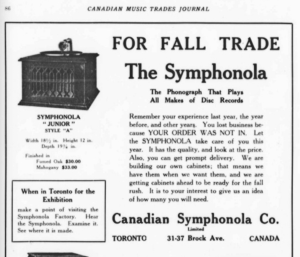
It appears to be a “Junior” model from a company called the Canadian Symphonola Co., Limited, which had a factory and headquarters at 31-37 Brock Avenue, Toronto.
This advertisement for the Junior is from the Canadian Music Trades Journal in August, 1917. Mine is the Fumed Oak variant.
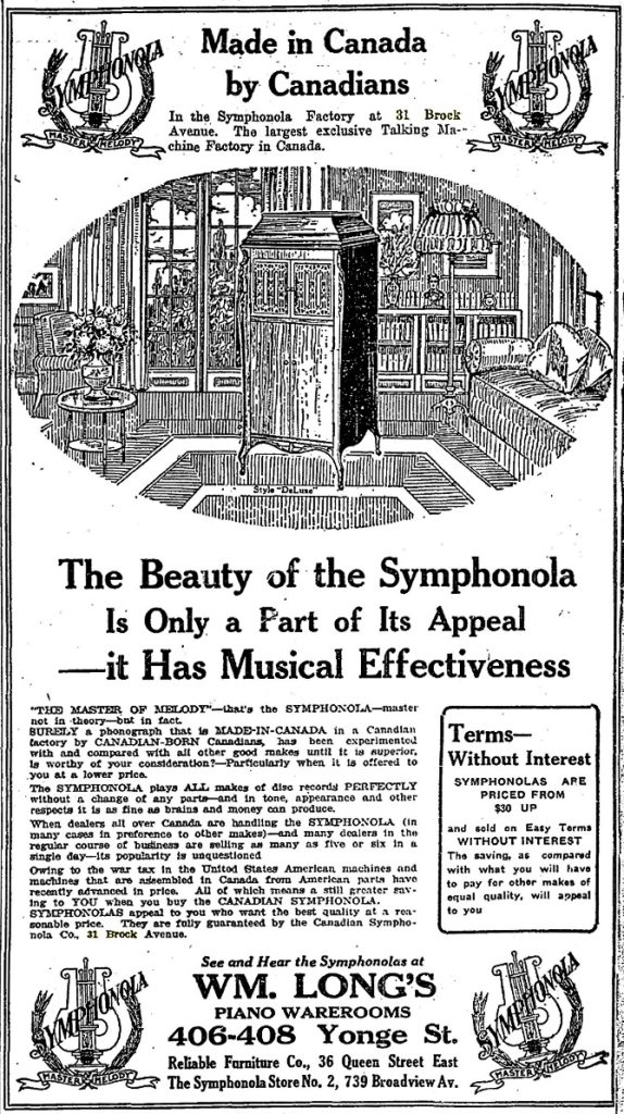
One interesting thing that I’ve come across when digging into this was this advertisement from the Toronto Daily Star in December, 1917.
The >100-year old text is weirdly familiar in these times of rather unstable international relationships. History has a tendency to rhyme.
For more information about the Symphonola company, this page at capsnews.org is a great resource. (it’s also where I found those two screenshots above…)
One of my favourite pithy quotes is ‘Tradition is just peer pressure from dead people’. When you start looking at some of the things we ‘just do’, you start asking yourself ‘why, exactly?’
For example, when you attend a wedding, you’ll see the bride standing on the groom’s left. This is so that he can use his sword to fight off her family as he carries away from the town over his left shoulder.
Another example is the story that’s often told about how the distance between railway tracks is related to the width of a horse’s ass.
There’s a similar thing that happens in multichannel audio systems. When people ask me what I would recommend for loudspeakers when building a multichannel (or ‘surround’) system, I always start with the ITU’s Recommendation BS.775 which says that you should use matching loudspeakers all-round. Of course, almost no one does this, so the next best thing is to say something like the following:
use big loudspeakers for your Left Front and Right Front
use smaller (but matched) loudspeakers for your surround channels (including back and height channels)
make some intelligent choice about your Centre Front loudspeaker (which is not terribly helpful, but there are many issues to consider when thinking about your centre front loudspeaker)
This raises a question:
‘Why is it okay to use smaller, less capable loudspeakers for the surround channels?’
The simple answer to this is that for most materials, there isn’t as much signal in the surround channels, and there’s certainly less low-frequency, high-level content.
However, let’s keep asking questions:
‘Why isn’t there more content (in terms of both bandwidth and level) in the surround and height channels?’
The answer to this is that surround sound (like stereo, which is in effect the same thing) originated with movies. The first big blockbuster that was released in Dolby Stereo (later re-branded as Dolby Surround) was Star Wars in 1977 or so. Dolby Stereo was a 4-2-4 ‘encoding’ system that relied heavily on M-S encoding and decoding. If I over-simplify this a little, then the basic idea was:
The Centre channel was sent to both the Left and Right channels on the film
Left channel was sent to Left
Right channel was sent to Right
The Surround channel (there was only one) was mixed into the Left and Right channels in opposite polarity (aka ‘out of phase’)
So, the re-recording engineer (the film world’s version of a recording engineer) mixed in a 4-channel world: Left, Right, Centre, and Surround, but the film only contained two channels: Left Total and Right Total (with the Centre and Surround content mixed in them).
When the film was shown in a theatre with a Dolby Stereo decoder, the two channels on the film were ‘decoded’ to the original four channels and send out to the loudspeakers in the cinema.
This was a great concept based on an old idea, since M-S processing was part of Blumlein’s original patent for stereo back in 1931. When you’re looking at a two-channel stereo signal, you can think of it as independent Left and Right channels. However, usually, if you look at the content, the two channels contain related information. For example, the lead vocal of almost every pop tune is identical in the Left and Right channels so that its phantom image appears in the centre.
So, another way of thinking of the same two-channel stereo signal is by considering the two channels as
‘M’ (for Mid or Mono, depending on which book you read): the signal that is identical in the Left and Right
‘S’ (for Side or Stereo): the signal that is identical except in opposite polarity in the Left and Right
For example, FM Stereo is not sent as Left and Right channels, it’s sent as M and S channels. There’s less bandwidth and less level in the S component, so when you lose the FM signal to your antenna, the first thing to go is the S, and you’re left with a Mono radio station.
Wait… there’s that ‘less bandwidth and less level in the S component’ again – just like what I said above about the surround channels in a surround system.
Let’s back up a little to vinyl records. A groove of a vinyl record is a 90º cut, with the needle resting gently on both walls of that trough. If the left wall moves up and down (on a 45º angle to the surface of the vinyl) then the needle bounces up and down with it, but only for that left channel. In other words, it slides along the right wall of the tough.
When a signal is the same in the left and right channels on a vinyl record (the M-component, like the lead vocal) then, when one side of the groove pushes the needle UP, the other side drops DOWN. This means that the M-component signal results in the needle moving horizontally (or laterally), in parallel with the surface of the disc. Signals in the S-component (when the Left and Right channels are ‘out of phase’) result in the two walls moving upwards and downwards together, pushing the needle vertically.
The reason for this is that the old mono shellac discs used laterally-cut grooves, and the reason for this was (apparently) that Emile Berliner was getting around a Thomas Edison patent. Also, by making the needle sensitive to lateral movements, it was less sensitive to vibrations caused by footsteps, which primarily cause the gramophone to vibrate vertically. When they made the first two-channel discs, it was smart to make the format backwards-compatible with Berliner’s existing gramophones.
So, if you have a lot of level and a lot of low-frequency content in the signal on a vinyl record, it causes the needle to jump up and down, and it will likely get thrown out of the groove and cause the record to skip. This is why the bass on vinyl records has to be monophonic, even though the record itself is two-channel stereo. Mono bass causes the needle to wiggle left-right, but not up-down.
So, the historically-accurate answer to explain why it’s okay to use smaller loudspeakers for most of the outputs in a modern 7.1.4 system is that we are maintaining compatibility with a format from 1892.
Another gem of historical information from the Centennial Issue of the JAES in 1977.
This one is from the article titled “The Recording Industry in Japan” by Toshiya Inoue of the Victor Company of Japan. In it, you can find the following:
Notice that this describes a 3-channel system developed by the Victor Company using FM with a carrier frequency of 24 kHz and a modulation of ±4kHz to create a third channel on the vinyl. The resulting signal had a bandwidth of 50 Hz to 5 kHz and a SNR of 47 dB.
Interestingly, this was developed from 1961-1965: starting 9 years before CD-4 quadraphonic was introduced to the market, which used the same basic principle of FM modulation to encode the extra channels.
This episode of The Infinite Monkey Cage is worth a listen if you’re interested in the history of recording technologies.
There’s one comment in there by Brian Eno that I COMPLETELY agree with. He mentions that we invented a new word for moving pictures: “movies” to distinguish them from the live equivalent, “plays”. But we never really did this for music… Unless, of course, you distinguish listening to a “concert” from listening to a “recording” – but most of us just say “I’m listening to music”.
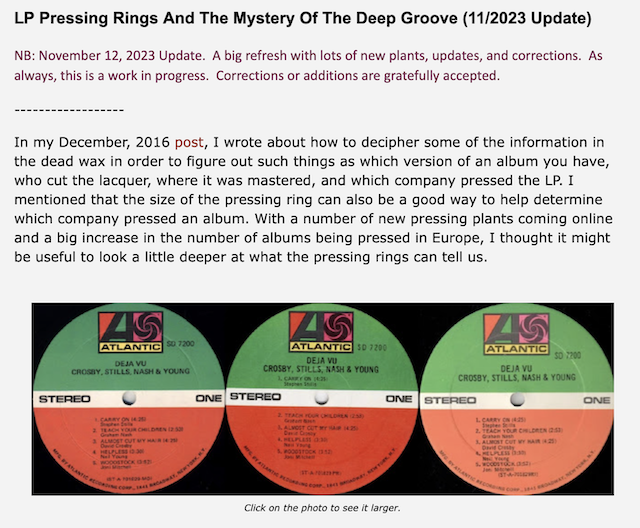
If you have a vinyl record, and you’re curious about where in the world it was pressed, this site might have some information to help you trace its roots.
I had a little time at work today waiting for some visitors to show up and, as I sometimes do, I pulled an old audio book off the shelf and browsed through it. As usually happens when I do this, something interesting caught my eye.
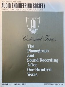
I was reading the AES publication called “The Phonograph and Sound Recording After One-Hundred Years” which was the centennial issue of the Journal of the AES from October / November 1977.
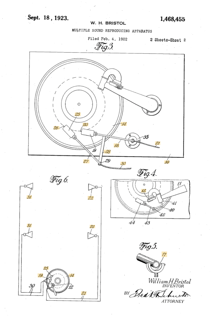
In that issue of the JAES, there is an article called “Record Changers, Turntables, and Tone Arms – A Brief Technical History” by James H. Kogen of Shure Brothers Incorporated, and in that article he mentions US Patent Number 1,468,455 by William H. Bristol of Waterbury, CT, titled “Multiple Sound-Reproducing Apparatus”.
Before I go any further, let’s put the date of this patent in perspective. In 1923, record players existed, but they were wound by hand and ran on clockwork-driven mechanisms. The steel needle was mechanically connected to a diaphragm at the bottom of a horn. There were no electrical parts, since lots of people still didn’t even have electrical wiring in their homes: radios were battery-powered. Yes, electrically-driven loudspeakers existed, but they weren’t something you’d find just anywhere…
In addition, 3- or 2-channel stereo wasn’t invented yet, Blumlein wouldn’t patent a method for encoding two channels on a record until 1931: 8 years in the future…
But, if we look at Bristol’s patent, we see a couple of astonishing things, in my opinion.
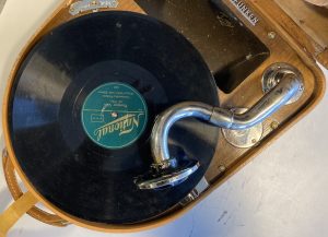
If you look at the top figure, you can see the record, sitting on the gramophone (I will not call it a record player or a turntable…). The needle and diaphragm are connected to the base of the horn (seen on the top right of Figure 3, looking very much like my old Telefunken Lido, shown below.
But, below that, on the bottom of Figure 3 are what looks a modern-ish looking tonearm (item number 18) with a second tonearm connected to it (item number 27). Bristol mentions the pickups on these as “electrical transmitters”: this was “bleeding edge” emerging technology at the time.
So, why two pickups? First a little side-story.
Anyone who works with audio upmixers knows that one of the “tricks” that are used is to derive some signal from the incoming playback, delay it, and then send the result to the rear or “surround” loudspeakers. This is a method that has been around for decades, and is very easy to implement these days, since delaying audio in a digital system is just a matter of putting the signal into a memory and playing it out a little later.
Now look at those two tonearms and their pickups. As the record turns, pickup number 20 in Figure 3 will play the signal first, and then, a little later, the same signal will be played by pickup number 26.
Then if you look at Figure 6, you can see that the first signal gets sent to two loudspeakers on the right of the figure (items number 22) and the second signal gets sent to the “surround” loudspeakers on the left (items number 31).
So, here we have an example of a system that was upmixing a surround playback even before 2-channel stereo was invented.
Mind blown…
NB. If you look at Figure 4, you can see that he thought of making the system compatible with the original needle in the horn. This is more obvious in Figures 1 and 2, shown below.
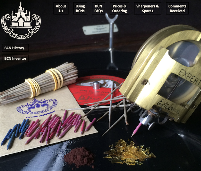
Once-upon-a-time I posted a little thing about Burmese Colour Needles for grammophones. Then, today, I received an email from the owner of www.burmesecolourneedles.com a company owned by Andy Briggs, where you can buy brand new ones!
Andy also has a YouTube channel that is well worth visiting.
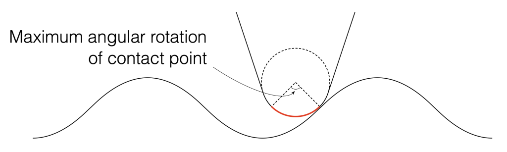
In the last posting, I showed a scale drawing of a 15 µm radius needle on a 1 kHz sine tone with a modulation velocity of 50 mm/s (peak) on the inside groove of a record. Looking at this, we could see that the maximum angular rotation of the contact point was about 13º away from vertical, so the total range of angular rotation of that point would be about 27º.
I also mentioned that, because vinyl is mastered so that the signal on the groove wall has a constant velocity from about 1 kHz and upwards, then that range will not change for that frequency band. Below 1 kHz, because the mastering is typically ensuring a constant amplitude on the groove wall, then the range decreases with frequency.
We can do the math to find out exactly what the angular rotation the contact point is for a given modulation velocity and groove speed.
Figure 1: A scale drawing of a 15 µm radius needle on a 1 kHz sine tone with a modulation velocity of 50 mm/s (peak) on the inside groove of a record. These two points are the two extremes of the angular rotation of the contact point.
Looking at Figure 1, the rotation is ±13.4º away from vertical on the maximum; so the total range is 26.8º. We convert this to a time modulation by converting that angular range to a distance, and dividing by the groove speed at the location of the needle on the record.
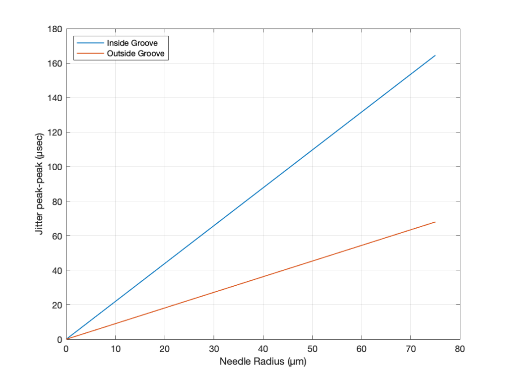
If we repeat that procedure for a range of needle radii from 0 µm to 75 µm for the best-case (the outside groove) and the worst-case (the inside groove), we get the results shown in Figure 2.
Figure 2. The peak-to-peak equivalent “jitter” values of the inside and outside grooves for a range of needle radii.
Back in Part II of what is turning out to be a series of postings on this topic, I wrote
If this were a digital system instead of an analogue one, we would be describing this as ‘signal-dependent jitter’, since it is a time modulation that is dependent on the slope of the signal. So, when someone complains about jitter as being one of the problems with digital audio, you can remind them that vinyl also suffers from the same basic problem…
As I was walking the dog on another night, I got to thinking whether it would be possible to compare this time distortion to the jitter specifications of a digital audio device. In other words, is it possible to use the same numbers to express both time distortions? That question led me here…
Remember that the effect we’re talking about is caused by the fact that the point of contact between the playback needle and the surface of the vinyl is moving, depending on the radius of the needle’s curvature and the slope of the groove wall modulation. Unless you buy a contact line needle, then you’ll see that the radius of its curvature is specified in µm – typically something between about 5 µm and 15 µm, depending on the pickup.
Now let’s do some math. The information and equations for these calculations can be found here.
We’ll start with a record that is spinning at 33 1/3 RPM. This means that it makes 0.556 revolutions per second.
The Groove Speed relative to the needle is dependent on the rotation speed and the radius – the distance from the centre of the record to the position of the needle. On a 12″ LP, the groove speed at the outside groove where the record starts is 509.8 mm/sec. At the inside groove at the end of the record, it’s 210.6 mm/sec.
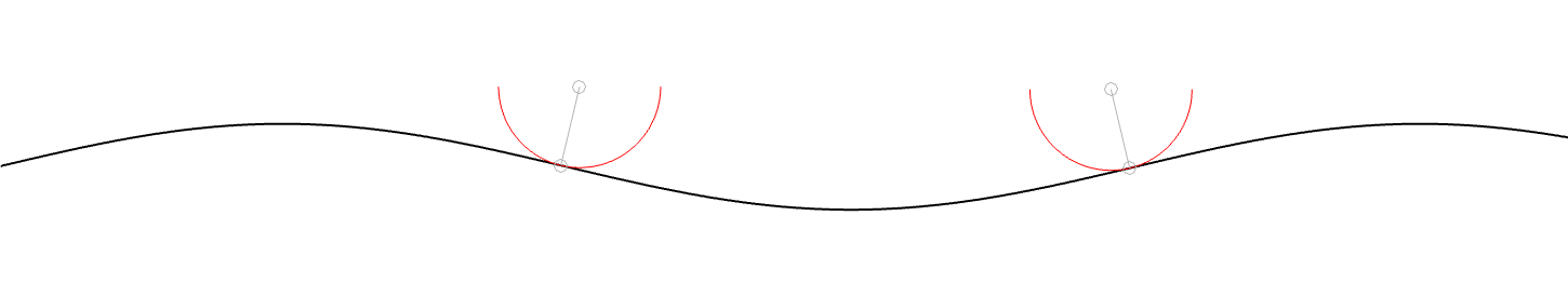
Let’s assume that the angular rotation of the contact point (shown in Figure 1) is 90º. This is not based on any sense of scale – I just picked a nice number.
Figure 1. Artists rendition of the range of the point of contact between the surface of the vinyl and the pickup needle.
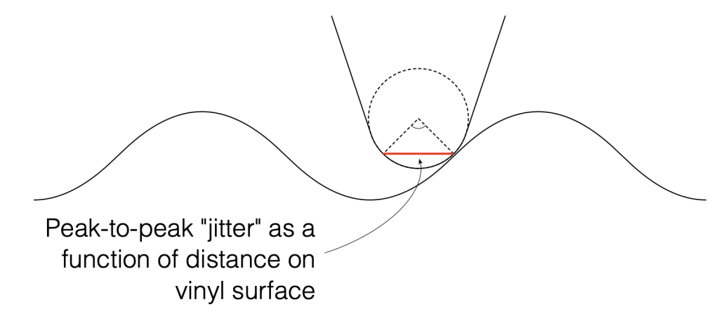
We can convert that angular shift into a shift in distance on the surface of the vinyl by finding the distance between the two points on the surface, as shown below in Figure 2. Since you might want to choose an angular rotation that is not 90º, you can do this with the following equation:
2 * sin(AngularRotation / 2) * radius
So, for example, for a needle with a radius of 10 µm and a total angular rotation of 90º, the distance will be:
2 * sin(90/2) * 10 = 14.1 µm
Figure 2. The angular range from Figure 1 converted to a linear distance on the vinyl’s surface.
We can then convert the “jitter” as a distance to a jitter in time by dividing it by the distance travelled by the needle each second – the groove speed in µm per second. Since that groove speed is dependent on where the needle is on the record, we’ll calculate it as best-case and a worst-case values: at the outside and the inside of the record.
Jitter Distance / Groove Speed = Jitter in time
For example, at the inside of the record where the jitter is worst (because the wavelength is shortest and therefore the maximum slope is highest), the groove speed is about 210.6 mm/sec or 210600 µm/sec.
Then the question is “what kind of jitter distance should we really expect?”
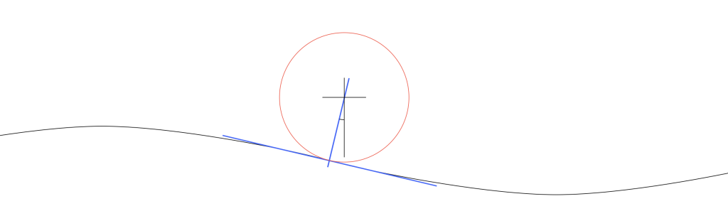
Figure 3. Scale drawing of a needle on a record.
Looking at Figure 3 which shows a scale drawing of a 15 µm radius needle on a 1 kHz tone with a modulation velocity of 50 mm/s (peak) on the inside groove of a record, we can see that the angular rotation at the highest (negative) slope is about 13.4º. This makes the total range about 27º, and therefore the jitter distance is about 7.0 µm.
If we have a 27º angular rotation on a 15 µm radius needle, then the jitter will be
7.0 / 210600 = 0.0000332 or 33.2 µsec peak-to-peak
Of course, as the radius of the needle decreases, the angular rotation also decreases, and therefore the amount of “jitter” drops. When the radius = 0, then the jitter = 0.
It’s also important to note that the jitter will be less at the outside groove of the record, since the wavelength is longer, and therefore the slope of the groove is lower, which also reduces the angular rotation of the contact point.
Since the groove on records are typically equalised to ensure that you have a (roughly) constant velocity above 1 kHz and a constant amplitude below, then this means that the maximum slope of the signal and therefore the range of angular rotation of the contact point will be (roughly) the same from 1 kHz to 20 kHz. As the frequency of the signal descended from 1 kHz and downwards, the amplitude remains (roughly) the same, so the velocity decreases, and therefore the range of the angular rotation of the contact point does as well.
In other words, the amount of jitter is 0 at 0 Hz, and increases with frequency until about 1 kHz, then it remains the same up to 20 kHz.
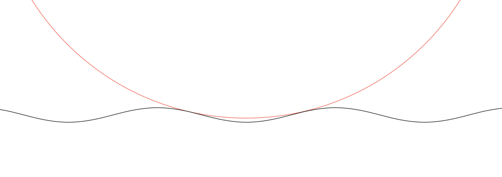
As one final thing: as I was drawing Figure 3, I also did a scale drawing of a 20 kHz signal with the same 50 mm/s modulation velocity and the same 15 µm radius needle. It’s shown in Figure 4.
Figure 4. Scale drawing of a needle on a record.
As you can see there, the needle’s 15 µm radius means that it can’t drop into the trough of the signal. So, that needle is far too big to play a CD-4 quad record (which can go all the way up to 45 kHz).


.jpg)