Let’s say that, for some reason, you want to apply an equaliser to an audio signal. It doesn’t matter why you want to do this: maybe you like more bass, maybe you need more treble, maybe you’re trying to reduce the audibility of a room mode. However, one thing that you should know is that, by changing the frequency response of the system, you are also changing its time response.

Now, before we go any farther, do NOT mis-interpret that last sentence to mean that a change in the time response is a bad thing. Maybe the thing you’re trying to fix already has an issue with its time response, and sometimes you have to fight fire with fire.

Before we start talking about filters, let’s talk about what “time response” means. I often work in an especially-built listening room that has acoustical treatments that are specifically designed and implemented to result in a very controlled acoustical behaviour. I often have visitors in there, and one of the things they do to “test the acoustics” is to clap their hands once – and then listen.

On the one hand (ha ha) this is a strange thing to do, because the room is not designed to make the sound of a single hand clap performed at the listening position sound “good” (whatever that means). On the other hand, the test is not completely useless. It’s a “play-toy” version of a very useful test we use to measure a loudspeaker called an impulse response measurement. The clap is an impulsive sound (a short, loud sound) and the question is “how does the thing you’re measuring (a room or a loudspeaker, for example) respond to that impulse?”

So, let’s start by talking about the two important reasons why we use an impulse.

Time response

If a thing in a room makes a sound, then the sound radiates in all directions and starts meeting objects in its path – things like walls and furniture and you. When that happens, the surface it meets will absorb some amount of energy and reflect the rest, and this is balance of absorbed-to-reflected energy is different at different frequencies. A cat will absorb high frequencies and low frequencies will just pass by it. A large flat wall made of gypsum will reflect high frequencies and absorb whatever frequency it “wants” to vibrate at when you thump it with your fist.

The energy that is absorbed is (eventually) converted to heat: that’s lost. The reflected energy comes back into the room and heads towards another surface – which might be you as well, but probably isn’t unless you’re in a room about the size of an ancient structure known to archeologists as a “phone booth”.

At your location, you only hear the sound that reaches you. The first part of the sound that you hear “immediately” after the thing made the noise, probably travelled a path directly from the source to you. Let’s say that you’re in a large church or an aircraft hangar – the last sound that you hear as it decays to nothing might be 5 seconds (or more!) after the thing made the noise, which means that the sound travelled a total of 5 sec * 344 m/s = 1.72 km bouncing around the church before finally arriving at your position.

So, if I put a loudspeaker that radiates simultaneously in all directions equally at all frequencies (audio geeks call this a point source) somewhere in a room, and I put a microphone that is equally sensitive to all frequencies from all directions (audio geeks call this an omnidirectional microphone) and I send an impulse (a “click”) out of the loudspeaker and record the output of the microphone, I’ll see something like this:

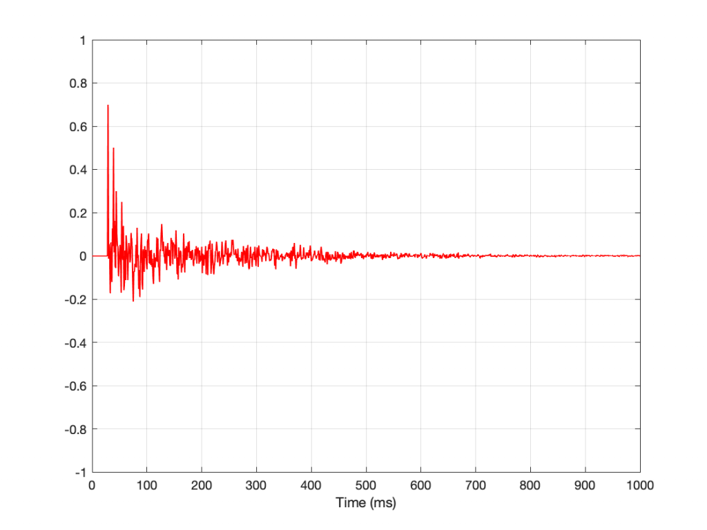
Some things to notice about that plot shown above

• There is some silence before the first sound starts. This is the time it takes for the sound to get from the loudspeaker to the microphone (travelling at about 344 m/s, and with an onset of about 30 ms, this means that the microphone was about 10.3 m away.
• There are some significant spikes in the signal after the first one. These are nice, clean reflections off some surfaces like walls, the floor or the ceiling.
• Mostly, this is a big mess, so it’s difficult to point somewhere else and say something like “that is the reflection off the coffee mug on the table over there, after the sound has already hit the ceiling and two walls on the way” for example…

So, this shows us something about how the room responds to an impulse over time. The nice (theoretical) thing is that this is a plot of what will happen to everything that comes out of the loudspeaker, over time, when captured at the microphone’s position. In other words, if you know the instantaneous sound pressure at any given moment at the output of the point-source loudspeaker, then you can go through time, multiplying that value by each value, moment by moment, in that plot to predict what will come out of the microphone. But this means that the total output of the microphone is all of the sound that came out of the loudspeaker over the 1000 ms plotted there, with each moment individually multiplied by each point on the plot – and all added together.

This may sound complicated, but think of it as a more simple example: When you’re sitting and listening to someone speak in a church, you can hear what that person just said, in addition to the reverberation (reflections) of what they said seconds ago. There is one theory that this is how harmony was invented: choirs in churches noticed that the reverb from the previous note blended nicely with the current note, and so chords were born.

Frequency Response

There is a second really good reason for using an impulse to test a system. An impulse (in theory) contains all frequencies at the same level. This is a little difficult to wrap ones head around (at least, it took me years to figure out why…) but let me try to explain.

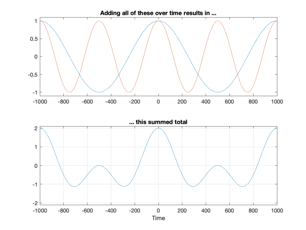
Any sound is the combination of some number of different frequencies, each with some level and some time relationship. This means that, I can start with the “ingredients” and add them together to make the sound I want. If I start with two frequencies: 1 Hz and 2 Hz and add them together, using cosine waves (a cosine wave is the same as a sine wave that starts 90º late), the result is as shown in Figure 2.

Let’s do this again, but increase the number to 5 frequencies: 1 Hz, 2 Hz, 3 Hz, 4 Hz, and 5 Hz.

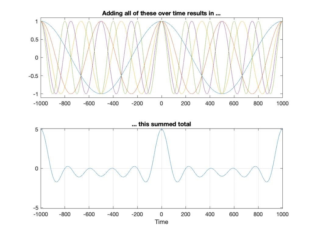
You may notice that the peak at Time = 0 ms is getting bigger relative to the rest of the result. However, we get the same peak values at Time = -1000 ms and Time = 1000 ms. This is because the frequencies I’m choosing are integer values: 1 Hz, 2 Hz, 3 Hz, and so on. What happens if we use frequencies in between? Say, 0.1 Hz to 10 Hz in steps of 0.1 Hz, thus making 100 cosine waves added together? Now they won’t line up nicely every second, so the result looks like Figure 4.

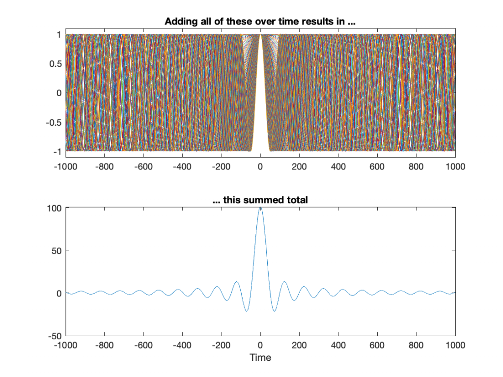
Let’s get crazy. Figure 5 shows 10,000 cosine waves with frequencies of 0 to 100 Hz in steps of 0.01 Hz.

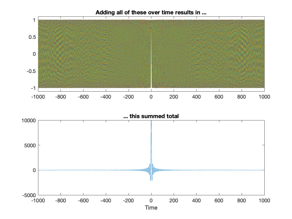
You may start to notice that the result of adding more and more cosine waves together at different frequencies is starting to look a lot like an impulse. It’s really loud at Time = 0 ms (whenever that is, but typically we think that it’s “now”) and it’s really quiet forever, both in the past and the future.

So, the moral of the story here is that if you click your fingers and make a “perfect” impulse, one philosophical way to think of this is that, at the beginning of time, cosine waves, all of them at different frequencies, started sounding – all of them cancelling each other until that moment when you decided to snap your fingers at Time = 0. Then they all continue until the end of time, cancelling each other out forever…

Or, another way to think of it is simply to say “an impulse contains all frequencies, each with the same amplitude”.

One small point: you may have noticed in Figure 5 that the impulse is getting big. That one added up to 10,001 – and we were just getting started. Theoretically, a real impulse is infinitely short and infinitely loud. However, you don’t want to make that sound because an infinitely loud sound will explode the universe, and that will wreck your analysis… It will at least clip your input.

Equalisation

Let’s take a simple example of an equaliser. I’ll use an EQ to apply a boost of 12 dB with a centre frequency of 1 kHz and a Q of 2. (Note that “Q” has different definitions. The one I’ll be using here is where the Q = Fc / BW, where BW is the bandwidth in Hz between the -3 dB points relative to the highest magnitude. If you want to dig deeper into this topic, you can start here.) That filter will have a magnitude response that looks like this:

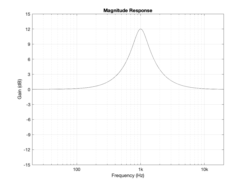
As you can see there, this means that a signal coming into that filter at 20 Hz or 20 kHz will come out at almost exactly the same level. At 1000 Hz, you’ll get 12 dB more at the output than the input. Other frequencies will have other results.

The question is: “how does the filter do that, conceptually speaking?”

That’s what we’ll look at in the next part of this series.