I’ve started working with a number of my colleagues on a series of videos for internal training at Bang & Olufsen. They were kind enough to make some of these videos publicly available.
This one is an explanation of the relationship between the frequency and the time domains, and why we often do “impulse response” measurements.
This posting is just wrapping up the series. No more plots… I promise.
Of course, this entire series has focused the “greatest hits” of the crossover club which is a limited number of crossover types. There are many other options that I haven’t talked about, but my point was not to explain how to choose and design a crossover for a loudspeaker for the DIY’er. It was to
give a primer on some of the things to consider when implementing a crossover
instil instinctive suspicion and doubt when you read an advertisement (or a comment on the Internet) that says something like “this loudspeaker is good (or bad) because it has THIS kind of crossover.”
There are plenty of things that I didn’t (and won’t) talk about, such as:
Crossovers for loudspeakers with more than two outputs
Other crossover designs. For example, as a start, search for:
Malcom Hawksford Asymmetrical Crossover
Malcom Hawksford discussion of stochastic crossovers associated with DMLs
On thing that I intentionally avoided was crossover designs that use filters with extremely high orders, sometimes called “brick wall” crossovers. On paper, they avoid the possible issues with a signal in a given frequency band coming from two sources (e.g. a woofer and a tweeter), so if you ONLY consider them from this perspective, they’re a good idea. However, in my opinion, this is outweighed by the facts that you will probably get a discontinuity in the power response (unless the two drivers have identical three-dimensional radiation patterns at the crossover frequency) AND you will probably have a complete mess in the time domain. Bonkers-order filters aren’t free. (If you clicked on the link to Linkwitz’s page, above and just taken a quick glance, then you’ve probably read the statement at the top of the page that says “The sum of acoustic lowpass and highpass outputs must have allpass behavior without high Q peaks in the group delay.” One way to look at the group delay of a filter is to look at the slope of the phase response. If you make a crossover with really high-order filters, then one of the artefacts will be a high slope in the phase response around the crossover frequency.)
One other thing that I have not mentioned is the incorrect naming that is often associated with crossovers and filters in general. Many people say “FIR Filter” (Finite Impulse Response) when they actually mean “Linear phase filter”. It’s important to remember that you can’t have a linear phase filter without an FIR filter implementation, but certainly not all FIR filters are linear phase. (Weirdly, a linear phase filter does, in fact, have an infinite impulse response, both forwards and backwards in time… But that’s a description of the filter’s response and not how it would be implemented in a DSP-based signal flow.) This incorrect usage drives me nuts. (Then again, many things like this do. For example, I get annoyed when HR people draw a triangle on a whiteboard and call it a pyramid. You never know what’s going to set me off on a pedantic rant about nomenclature.)
The other thing that I didn’t talk about was another way to look at a Butterworth two-way crossover, in which you see it as lacking a component in the s-domain (using Laplace analysis), which is the reason its sum has an allpass characteristic. If you add the missing component (for example, using a third loudspeaker driver), then the allpass behaviour disappears. This is the concept behind Bang & OIufsen’s “Uni-phase” series of loudspeakers in the 1970s and 1980s. If you want to learn more about this, I’ve already written about it here, and Erik Bækgaard’s original paper from 1977 describing the idea more fully can be found here.
Finally, hopefully, you won’t come away from all of this with a conclusion that one crossover is the winner. A crossover is just one component in a long series- and parallel-chain of components that make up a loudspeaker. Changing any of the other components may require making a different decision about another. And, in order to make that decision, you can’t just consider the on-axis response (unless you live alone in an anechoic chamber (or outdoors…). You also need to think about things like
the off-axis responses
the power response
the phase response
the time response and maybe also
the implications on latency
your required signal processing power (e.g. in MIPS)
maybe some other stuff if you have checked all those boxes.
On the other hand, after all this, you should also know that you can’t just implement a crossover ignoring everything else in the chain, and think that it’ll just work. It won’t.
Part 14 showed the power responses of a theoretical loudspeaker made with two point-sources using a linear-phase crossover using the method that I explained in Part 7.
In Part 11, I showed the power responses when the loudspeaker is made with real drivers in a real enclosure.
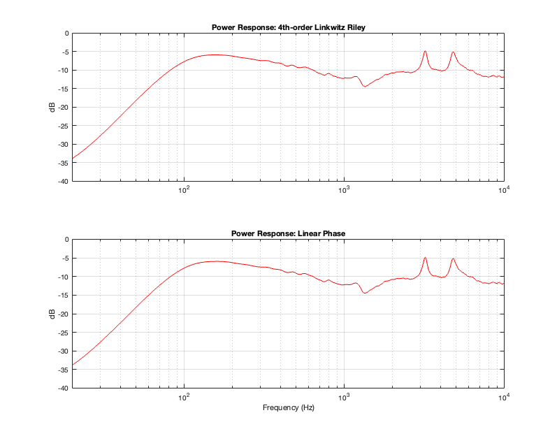
This posting shows the same as Part 11, except that I’ve implemented the crossover (at 1 kHz) using linear phase filters (again, with a really long window to avoid any discussion) instead of minimum phase filters.
Figure 15.1
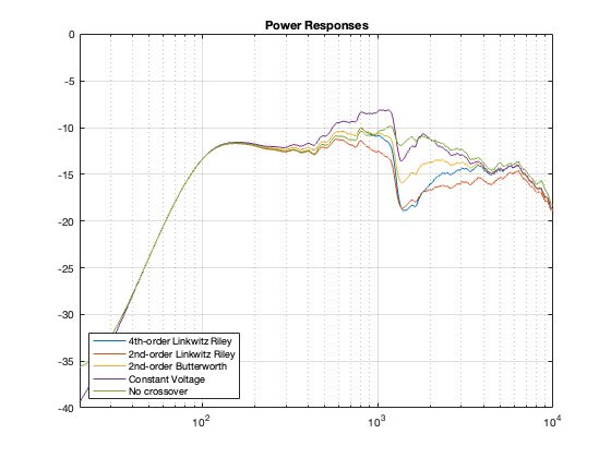
Figure 15.1 shows the real-world power responses of an actual two-way loudspeaker using two crossover strategies. (The top plot was already shown in Part 11.)
Based on the conclusions from Part 14, it should not come as a surprise that a linear phase crossover will result in the same power response as a 4th-order Linkwitz Riley crossover. The only reason I’m showing this here is to prove that the earlier conclusion based on a theoretical simulation holds true in real life.
One important conclusion to make at this point is to realise that a loudspeaker that is implemented with a 4th-order Linkwitz Riley crossover and the same loudspeaker implemented with a linear phase crossover will have identical magnitude responses (in any direction – not just on-axis) and identical power responses. However, they will have different phase responses (in any chosen direction) and different temporal responses (aka impulse responses).
In Part 7, I showed the power responses of three loudspeakers made with point-source (and therefore perfectly omnidirectional at all frequencies, which also means that they have the same response in all direction) drivers.
In that posting, I calculated the power response for a loudspeaker made of two loudspeaker drivers, floating in space, with the assumption that both drivers are point-sources, and that they do not live in an enclosure that has any acoustical effects. I also calculated the responses for 3 different distances between the drivers, which were chosen as a function of the crossover frequency’s wavelength.
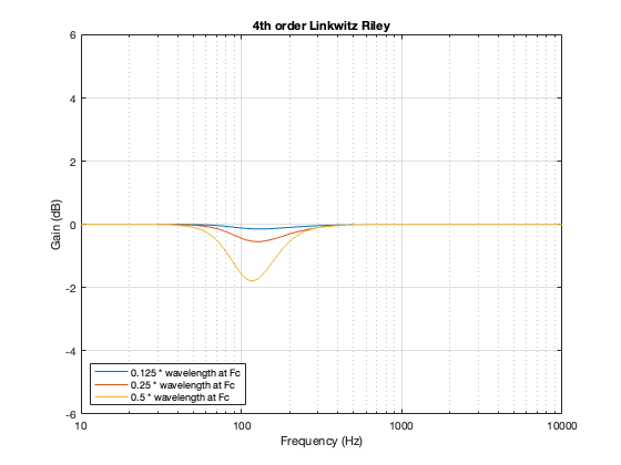
One of the crossover types whose power responses that I showed was the 4th-order Linkwitz Riley. The plots that I showed back then for that crossover type is reproduced here in Figure 14.1.
Figure 14.1: Power responses for a 2-way theoretical loudspeaker for three different distances between the drivers.
As I said, the details of how I calculated these power responses is detailed in Part 7.
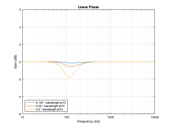
I calculated the power responses for a similar loudspeaker, using a linear phase crossover (with a really long window to avoid any discussion about this…) and with the same crossover frequency of 100 Hz and the same distances between the “drivers”. These power responses are shown below in Figure 14.2.
Figure 14.2: Power responses for a 2-way theoretical loudspeaker for three different distances between the drivers.
If you look at Figures 14.1 and 14.2 you could be forgiven for thinking that they look VERY similar. In fact, they’re essentially identical. This is because the 0º difference in phase caused by the linear phase crossover is the same as a 360º difference in phase caused by the 4th order Linkwitz Riley.
In other words, the message of this posting is that the power responses of a loudspeaker that has been implemented with a 4th order Linkwitz Riley crossover and the same loudspeaker with a linear phase crossover will have the same power responses, assuming that all other aspects of the loudspeaker are the same.
In the previous posting, I showed the frequency responses and impulse responses of the outputs of a crossover based on a linear phase filter strategy. One thing that can be seen in the impulse response plots in Figure 12.5 is that it never reaches a value of 0. It rings both backwards and forwards in time forever. However, this is not practical, since we don’t want to wait until the end of time to hear the output of our loudspeaker.
So, normally, we have to make a pragmatic choice about how long we’re willing to wait for the crossover filter’s to deliver an output. There are various ways to make this decision, but ultimately, we’re trying to balance the “error” in the responses of the crossover’s outputs with how long an input/output latency we’re willing to put up with. (We might also need to think about computational issues like how many calculations have to be done when you use a REALLY long filter, but I’m going to pretend that this is not an issue for this posting.)
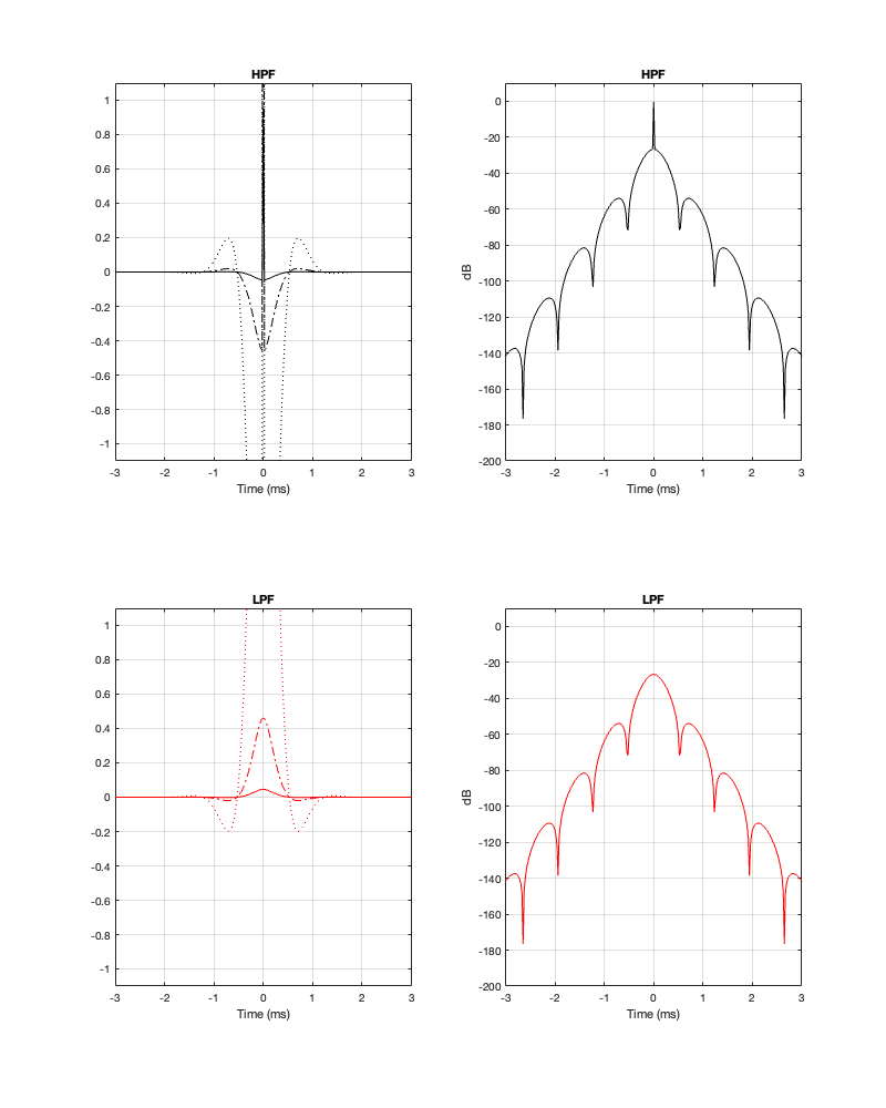
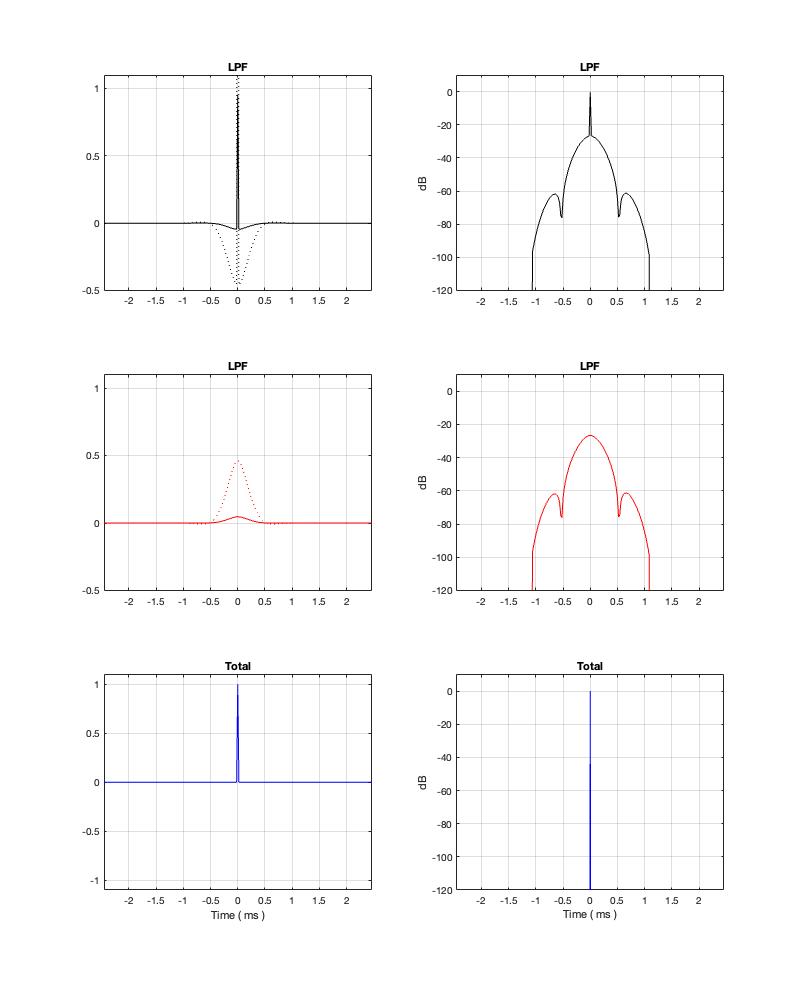
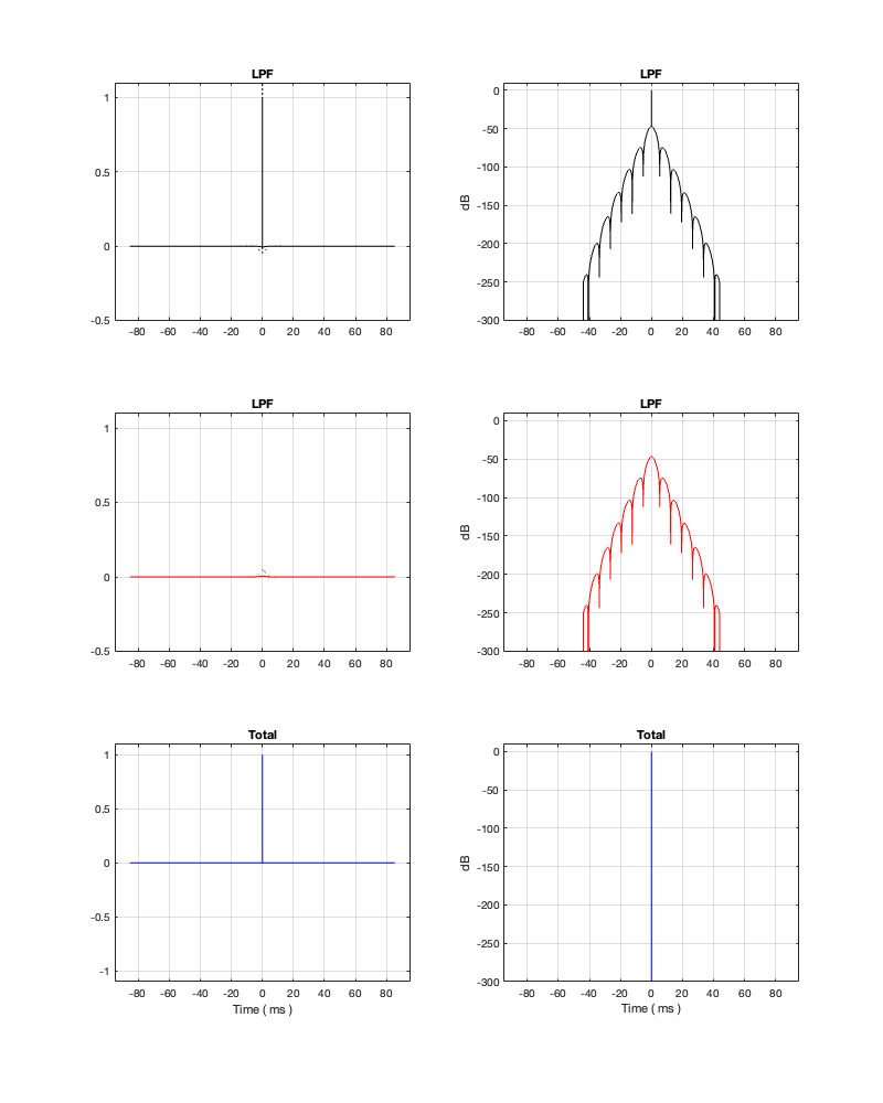
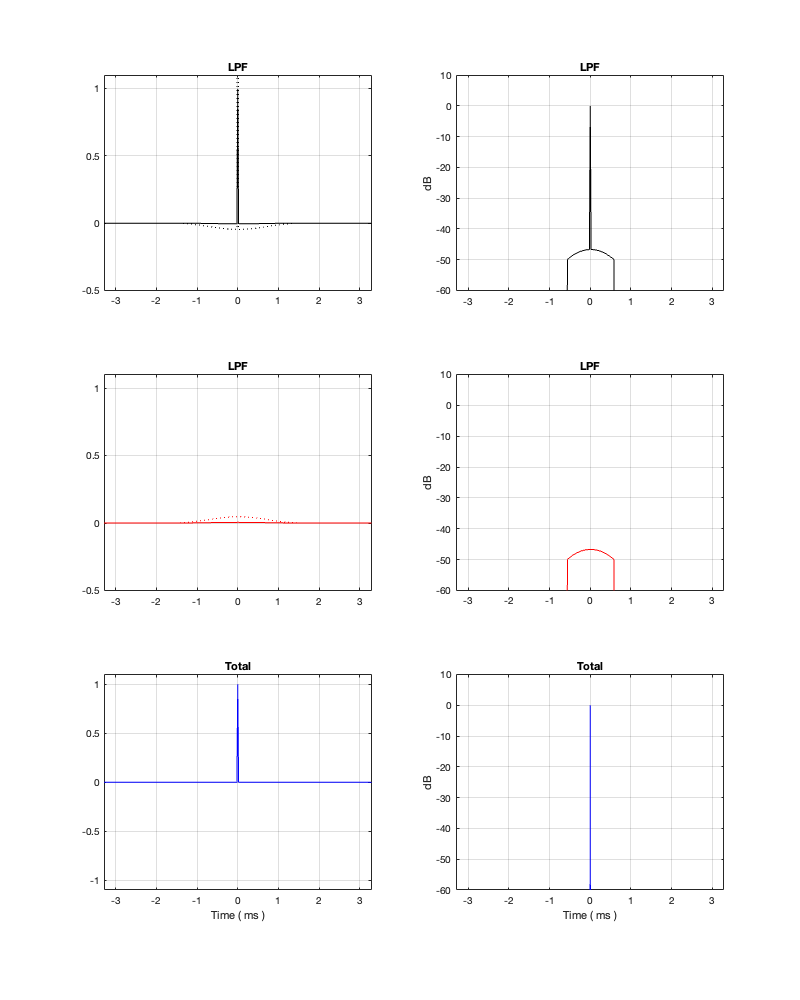
Figure 13.1. The left hand plots show the impulse responses of the two crossover outputs on three different scales: x1 (solid line), x10 (dash-dot line), and x100 (dotted line). The right-hand plots show the same impulse responses expressed in decibels.
It’s difficult to see from a linear plot of the impulse responses of the two filters, but the peak is in the middle, at Time = 0 ms. Extending outwards, both backwards and forwards in time, the impulse responses oscillates back and forth across the 0-amplitude line. This oscillation is easier to see when it’s plotted in decibels, but then you can’t see whether the linear value is positive or negative. So, it helps to look at both to get an idea of what’s happening.
One thing that might not be immediately obvious is that, apart from the big spike at Time = 0 ms on the high-pass filter response, the outputs of the two filters are identical in amplitude, but opposite in polarity. In other words, they are symmetrical. This makes sense when you consider that, by adding them together, the total result is a single spike at Time = 0 and an amplitude of 0 at all other times. In other other words, the outputs of the two filters “cancel each other out” at all times except Time = 0.
This is a little weird if you think of it as the tweeter cancelling the woofer – but you consider that it’s doing it in time, at very low levels, then it might make more intuitive sense.
What happens if you don’t want to wait too long to get the output? In other words, if we shorten the impulse response around the central spike? This is a technique that is called “windowing” where you slice a window of time out of the middle of the impulse response and use only that.
There are a number of ways to do this. We could just say “everything up to 1 ms before the spike and everything after 1 ms after the spike, we just convert to silence”. This is the simplest way to do it, but it’s also the dumbest.
A smarter way is to look at the impulse response shown above, and fade into the spike and then fade back out again. Then you just decide on the shape of the fade and its length. It could be a straight line, or it could be something fancy.
I’ve written a lot about windowing in another posting a long time ago. If you want to learn about this topic, you could start there, or any book or website that talks about time-domain processing and analysis of audio signals. I won’t explain windowing in this posting. It’ll just get too long…
For all of the analyses below I did the following:
Choose a crossover frequency
Implement the crossover using linear phase filters
Decide on a threshold in level (in dB below the spike at the input) to find out how long a window in time I’m going to use
Apply a Hann window to the filters’ impulse responses with the length that I found above
Show the magnitude and phase responses of the individual outputs as well as the summed total
Another way to do this would be to just decide on the length of the windowing (and find out the threshold of the level, below which you’re cutting the signal) and see what happens. Either way, you get a deviation in the response, you’re just setting a different parameter.
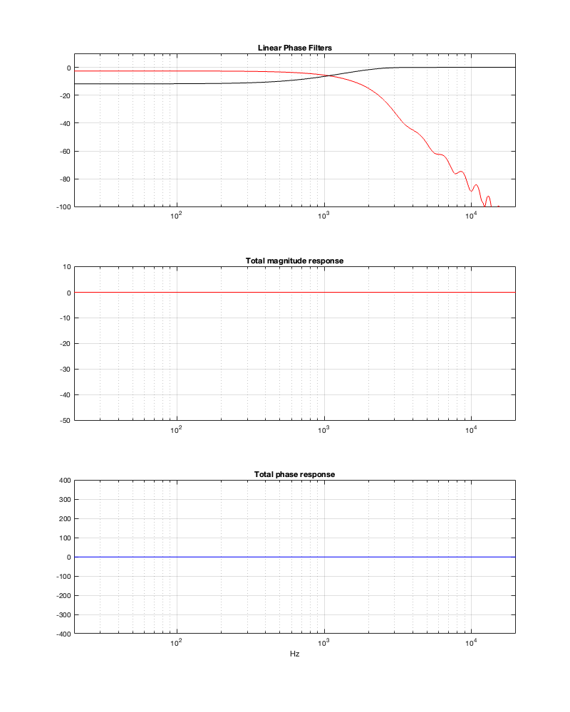
Fc = 1 kHz
Let’s start with a crossover frequency of 1 kHz. If I say that I want to extend the impulse response very far down in level, I’ll wind up getting a very accurate filter response (in other words, I’ll get what I expect), but it’ll have a long input/output latency (which is half of the total windowing time).
Figure 13.2. Fc = 1 kHz. Threshold = -250 dB Minimum Latency = 5.44 ms
Figure 13.3. Fc = 1 kHz. Threshold = -250 dB
Hopefully, comparing the plot in Figure 13.1 and 13.2 helps to clarify the explanation above. Essentially, the plots in those two figures show the same thing. However, you can see in Figure 13.2 that I’ve cut off the impulse response once it drops below -250 dB.
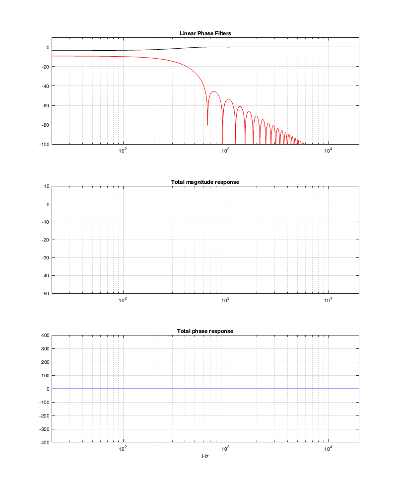
The effect of doing this windowing can be seen in Figure 13.3 where you can see that the roll-off for the tweeter doesn’t keep going down in level as you drop in frequency. This is because the lower the frequency you want to filter, the longer the filter’s impulse response has to be.
Notice, however, that, despite the fact that the two magnitude responses in the top of Figure 13.3 aren’t exactly what you’re expect, the responses of the summed total are what you’d expect. This will become a familiar theme as we continue.
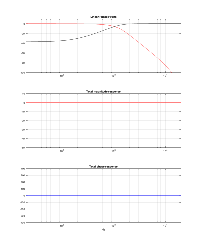
If we raise the threshold, we’ll shorten the impulse response, which means that we shorten the latency, and we deviate from the expected responses.
Figure 13.4: Fc = 1 kHz. Threshold = -100 dB Minimum Latency = 1.23 ms
Figure 13.5: Fc = 1 kHz. Threshold = -100 dB
Notice in Figure 13.5 that, although the two crossover outputs have very different magnitude responses from 13.3, the total sum still works. Intuitively, this actually makes sense when you look at the impulse responses, since they still cancel each other – they’re just identical but opposite (except for the spike in the tweeter).
Of course, since the filter is now shorter in time, we get a lot more low-frequency output from the tweeter.
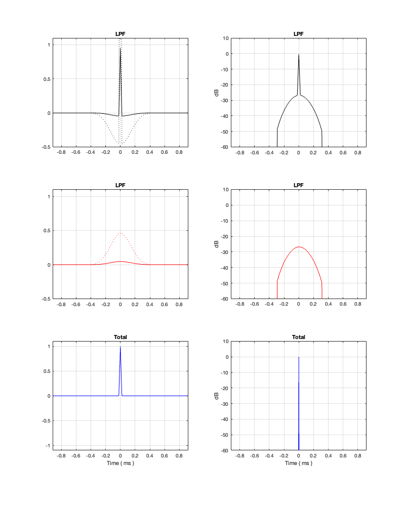
Figure 13.6: Fc = 1 kHz. Threshold = -50 dB Minimum Latency = 0.46 ms
Figure 13.7: Fc = 1 kHz. Threshold = -50 dB
Notice in Figures 13.6 and 13.7 that, with a threshold of -50 dB, our latency can be under 0.5 ms. However, we will be expecting a lot of level out of the tweeter at low frequencies, which might be unhealthy for it if we turn up the volume.
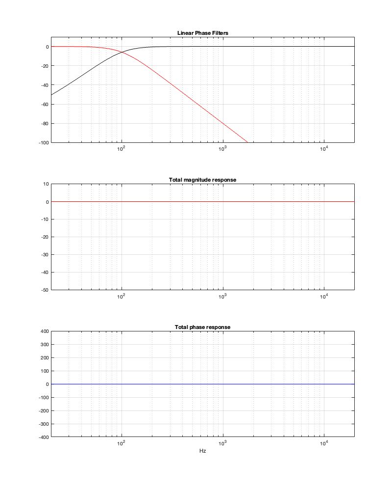
Fc = 100 Hz
Now let’s repeat the process with a 100 Hz crossover to see what happens.
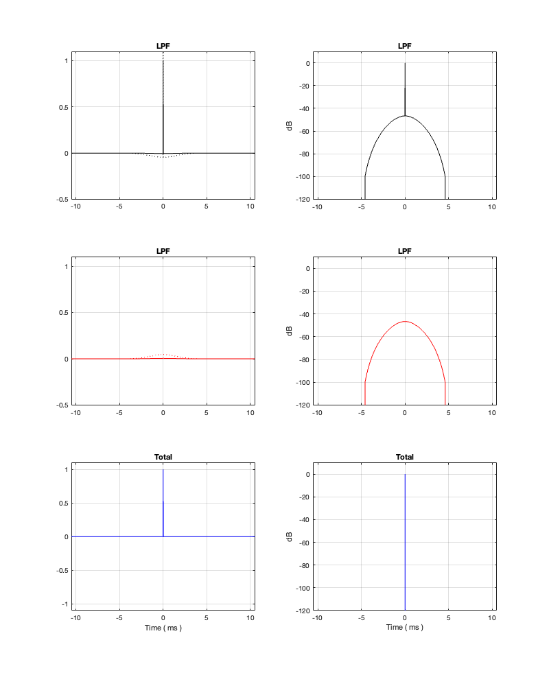
Figure 13.8: Fc = 100 Hz. Threshold = -250 dB Minimum Latency = 47.58 ms
Figure 13.9: Fc = 100 Hz. Threshold = -250 dB
Notice that, in order to implement a threshold of -250 dB, we need at least about 47 ms of latency, which is probably outside acceptable limits for lip synch with video. It’s certainly far too long to be used in a loudspeaker for live sound, since you’ll hear and echo-echo all the time-time.
Figure 13.10: Fc = 100 Hz. Threshold = -100 dB Minimum Latency = 5.27 ms
Figure 13.11: Fc = 100 Hz. Threshold = -100 dB
Notice that, by changing to a threshold of -100 dB, we’ve dropped our latency requirement significantly – down to just over 5 ms. However, don’t trust everything you see there. This crossover probably won’t behave nicely… If we change the threshold to -50 dB, you can see where we’re headed, and why I am highly suspicious of the -100 dB filters…
Figure 13.12: Fc = 100 Hz. Threshold = -50 dB Minimum Latency = 1.65 ms
Figure 13.13: Fc = 100 Hz. Threshold = -50 dB
Obviously, that filter isn’t going to give you what you want – although it’ll give it to you quickly… (Editorial comment: It’s like current AI: it’s the fastest way to get the wrong answer…)
Wrapping up for now
Like I said above, regardless of how much I shorten these impulse responses, the responses of the summed outputs look good. This doesn’t necessarily mean that the crossover will work well, as should be evident by looking at the responses of the individual outputs.
In addition, it should be evident that, in order to implement a linear phase crossover that behaves well, you will incur a latency that may not be acceptable, depending on the crossover frequency and your requirements. Then again, if you don’t care about latency, you might start requiring a lot of computational power to implement it.
Like any aspect of crossover choice and design, there are multiple parameters to play with…
In the next posting, we’ll take a look at the implications of a linear phase crossover on the three-dimensional power response.
Up to now in this series, we’ve looked at 4 different types of crossover designs:
4th-order Linkwitz Riley
2nd-order Linkwitz Riley
2nd-order Butterworth
One version of a Constant Voltage design
These have been interesting because they’re popular designs, and they are implementable using either analogue circuitry or digital signal processing (DSP). So, everything I’ve said so far is independent of whether the processing is analogue or digital. This is even true of all of those equalisers I applied to the two loudspeaker drivers to force them to be flat. Those are easiest to implement with DSP, but I didn’t do anything there that can’t be done with resistors, capacitors, and inductors.
But, the original question was
In passive crossovers, many are phase incoherent, meaning that the phase shift of one frequency will be different than another frequency. Do you agree? Am curious how this is dealt with in the active crossover’s of B&O products?
Hopefully, it’s obvious that the answer to the first question is “yes” – sort of… Passive crossovers are not “phase incoherent” – but they do have an effect on the phase response. As I’ve shown, you can think of the end result of a crossover implemented with minimum phase filters as an allpass filter. So there is an effect on the phase response of the loudspeaker. (Yes, the on-axis response of a Constant Phase crossover can result in a flat phase response, so that one might be an exception.)
However, if we leave analogue signal processing behind and go forwards limited to digital signal processing, then we have another option: linear phase filters.
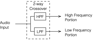
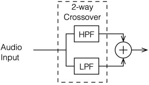
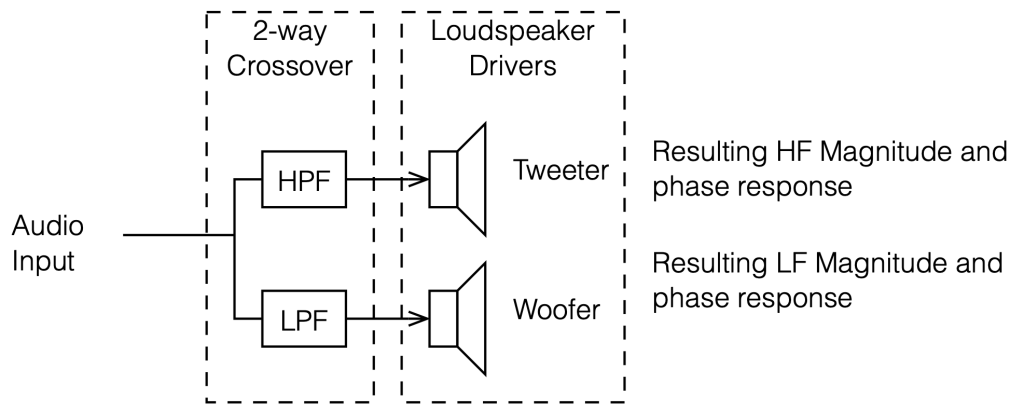
To start, let’s look at our original, simplified method of analysing a crossover, using the block diagrams shown in figures 12.1 and 12.2
Figure 12.1
Figure 12.2
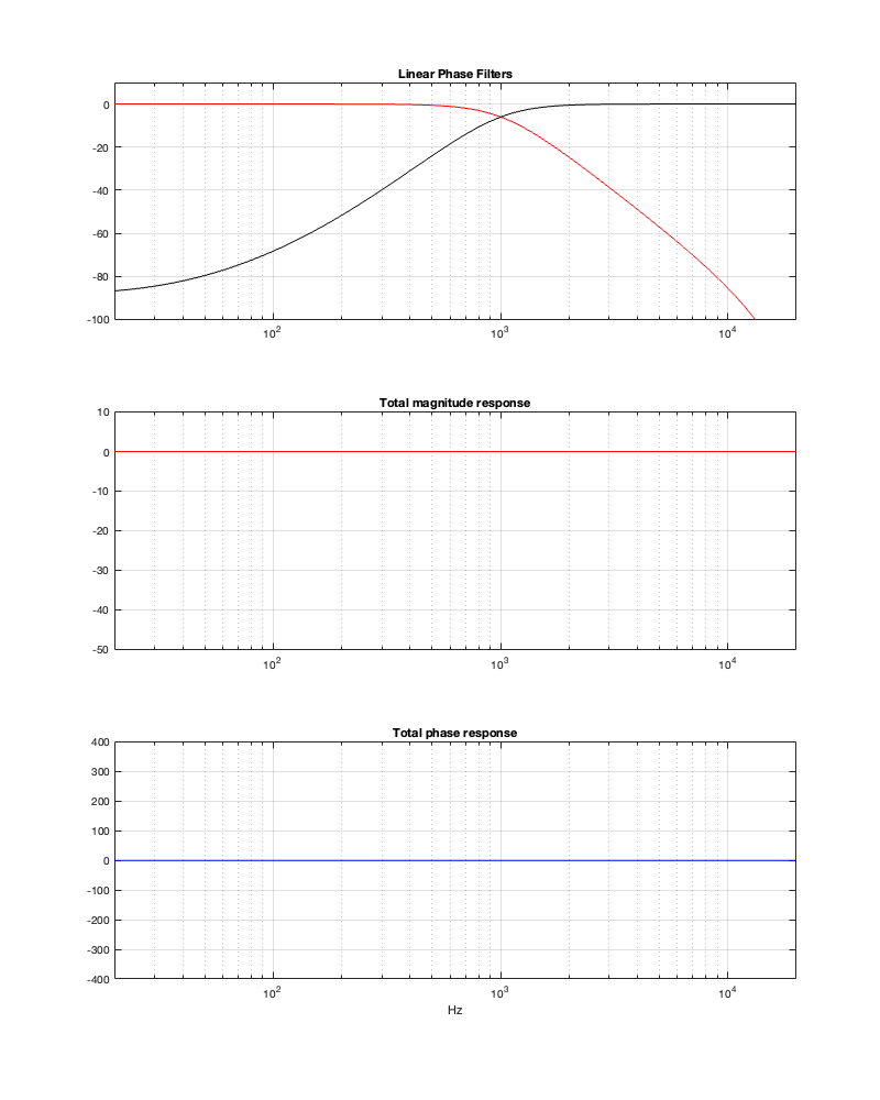
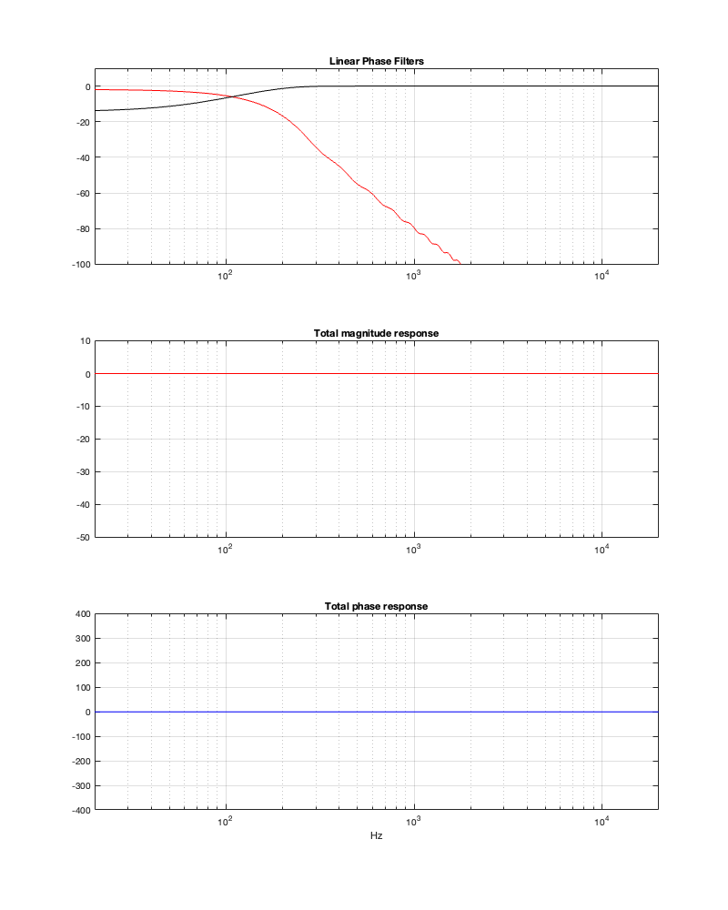
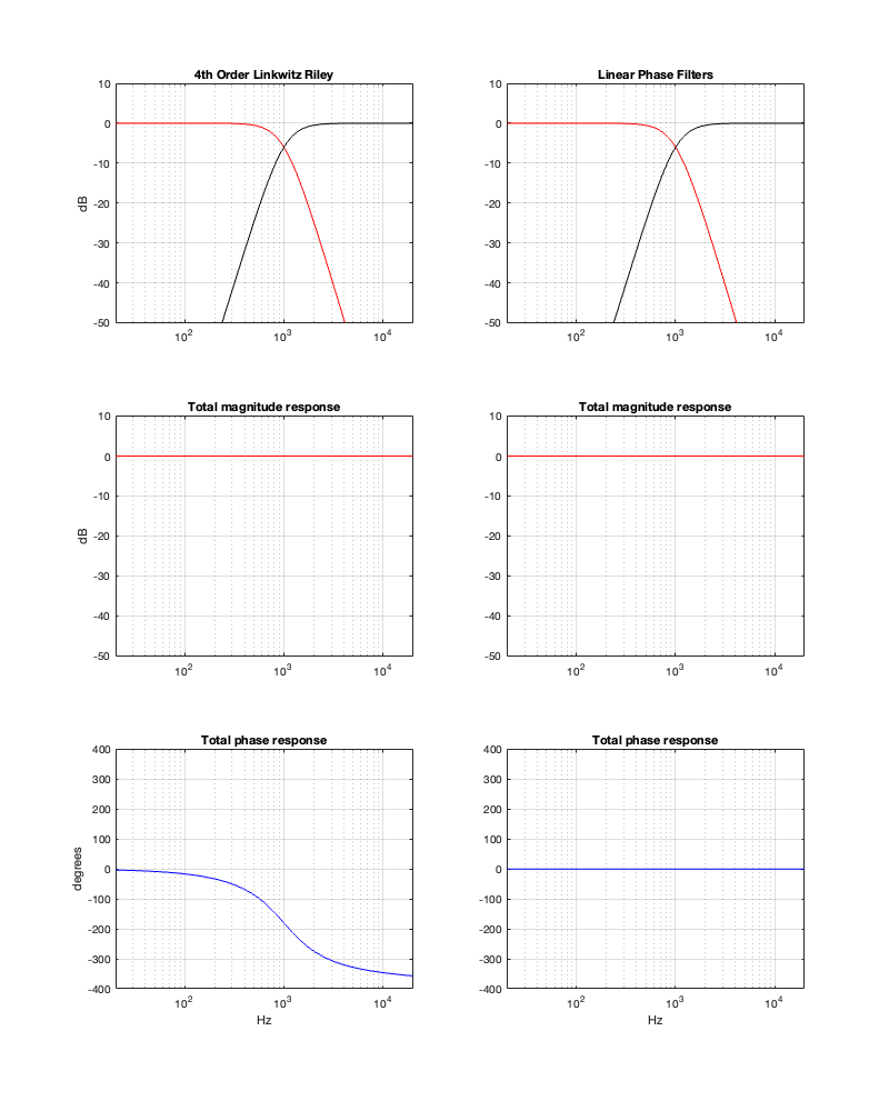
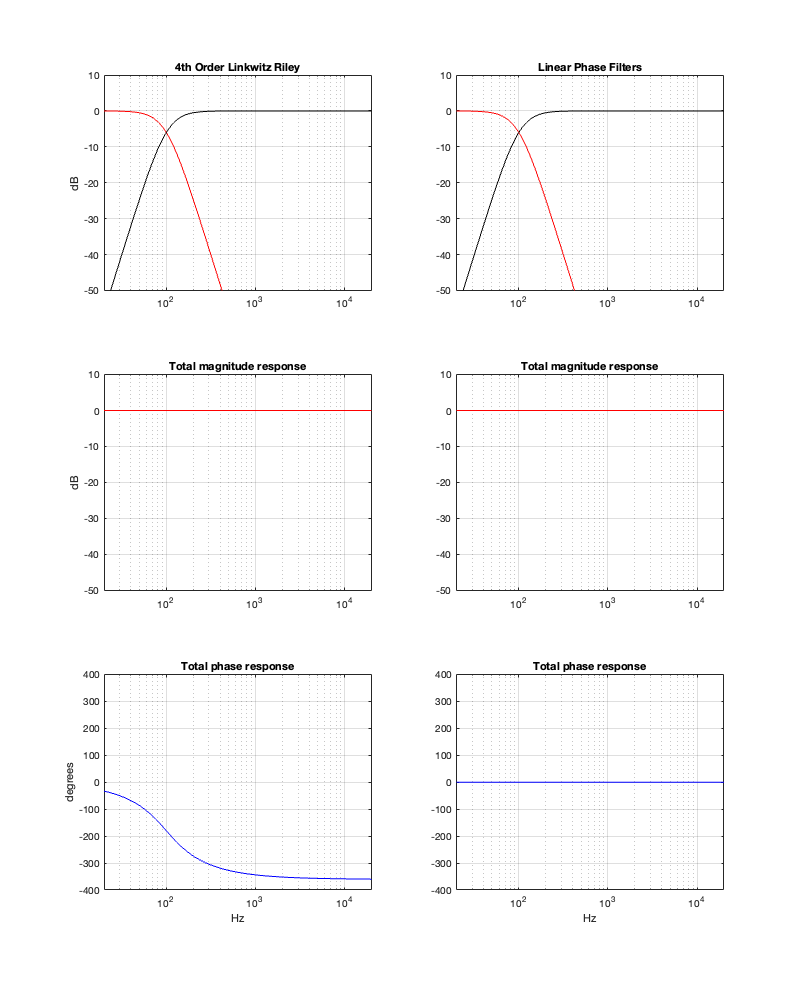
If we use this signal flow and create two crossovers at 1 kHz, one with a 4th-order Linkwitz Riley design (which I’ve already shown) and one with linear phase filters, the responses will look like the ones shown below in Figure 12.3
Figure 12.3: The magnitude and phase responses of two filters, one made with a 4th-order Linkwitz Riley design (on the left) and the other with linear phase filters (on the right)
Looking at the magnitude responses, you can see that these two filter designs are identical. However, the phase responses of their total outputs are not. The Linkwitz Riley design behaves like a minimum phase allpass filter, whereas the linear phase design does not.
So, this proves that a linear phase crossover is better, right? Not so fast… We’re not done yet…
Time response
The plots above show the frequency responses (“frequency response” is the combination of the magnitude response and the phase response) of the two designs. However, there is another way to look at the response of a system like a crossover, and that is to analyse how it behaves in time.
If we create a signal that is complete silence, and then a single one-sample-long “click”, we have something called an “impulse”. If we then send that into an audio system (like a crossover, for example), then we can see how it behaves in time – its temporal response. Since this method shows us how the system responds when you send an impulse through it, we call it the “impulse response” of the system.
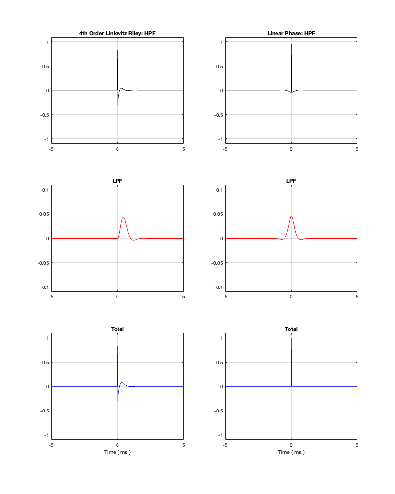
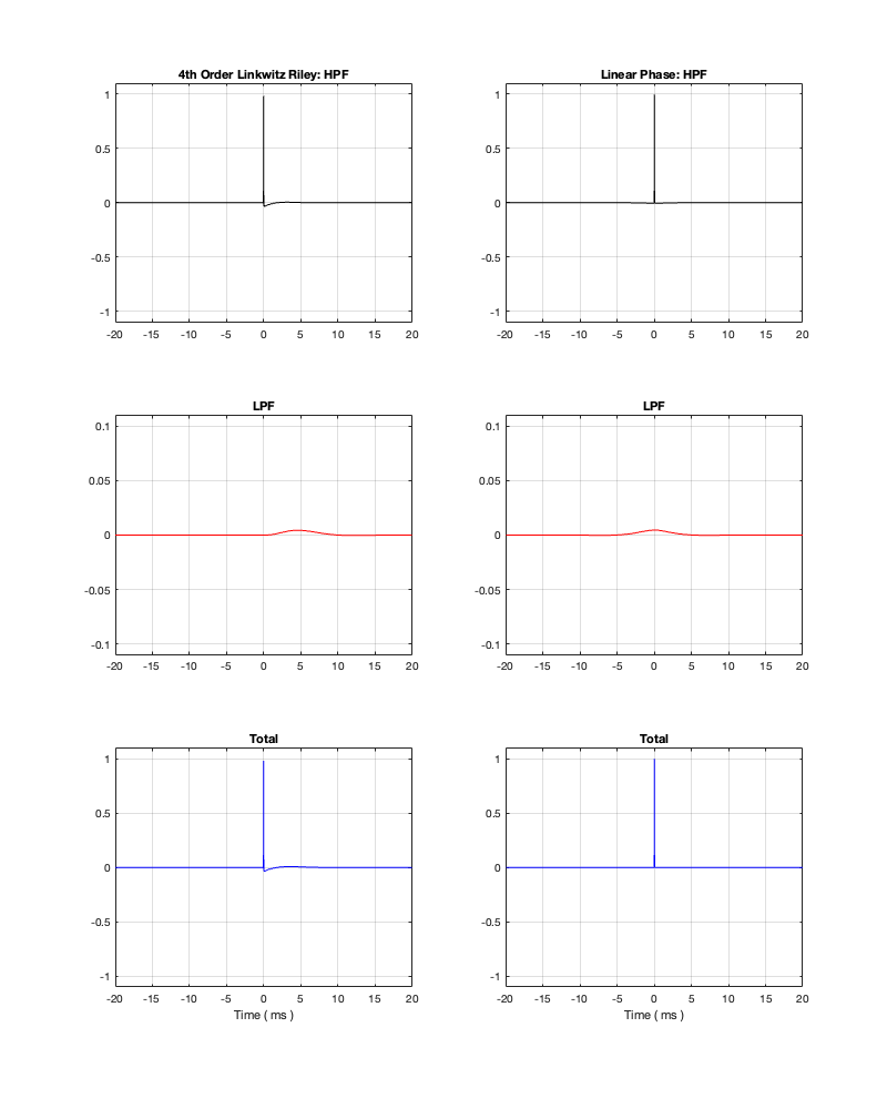
If we measure the impulse responses of our two 1 kHz crossovers, we get the results shown below in Figure 12.4.
Figure 12.4. The left-hand plots are the impulse responses for a 4th-order Linkwitz Riley crossover, the right-hand plots are for a linear phase crossover, both at 1 kHz.
As can be seen in the impulse response plots for the Linkwitz Riley crossover, until the impulse arrives at the input of the filter, the output of the filters are silence. This is the flat line with a constant amplitude of 0 from -5 ms to 0 ms. Then, at time = 0 ms, the impulse hits the input of the crossover, and something happens. The output of the high-pass filter spikes, and the output of the low-pass filter slowly (relatively speaking) starts ramping up. The combined output of the two filters, shown in blue, shows that the output is not a single-sample impulse. It has the characteristic shape of the impulse response of an all-pass filter.
The impulse responses of the high-pass and low-pass outputs of the linear phase crossover are similar-ish… but they have one characteristic that is VERY different. They have an output on the left side of time = 0 ms. One way to look at this is to say that they output a signal before the crossover gets something at its input. This is, of course, impossible: linear phase filters are not time machines.
So, how does this happen? By including a delay in the signal flow. In order to make a linear phase filter, you have to include a delay that starts is as long as is necessary to look after the stuff that you need to do to the signal before that big spike hits. So, if you want to use a linear-phase filter, then the “price” is that the output is going to be late.
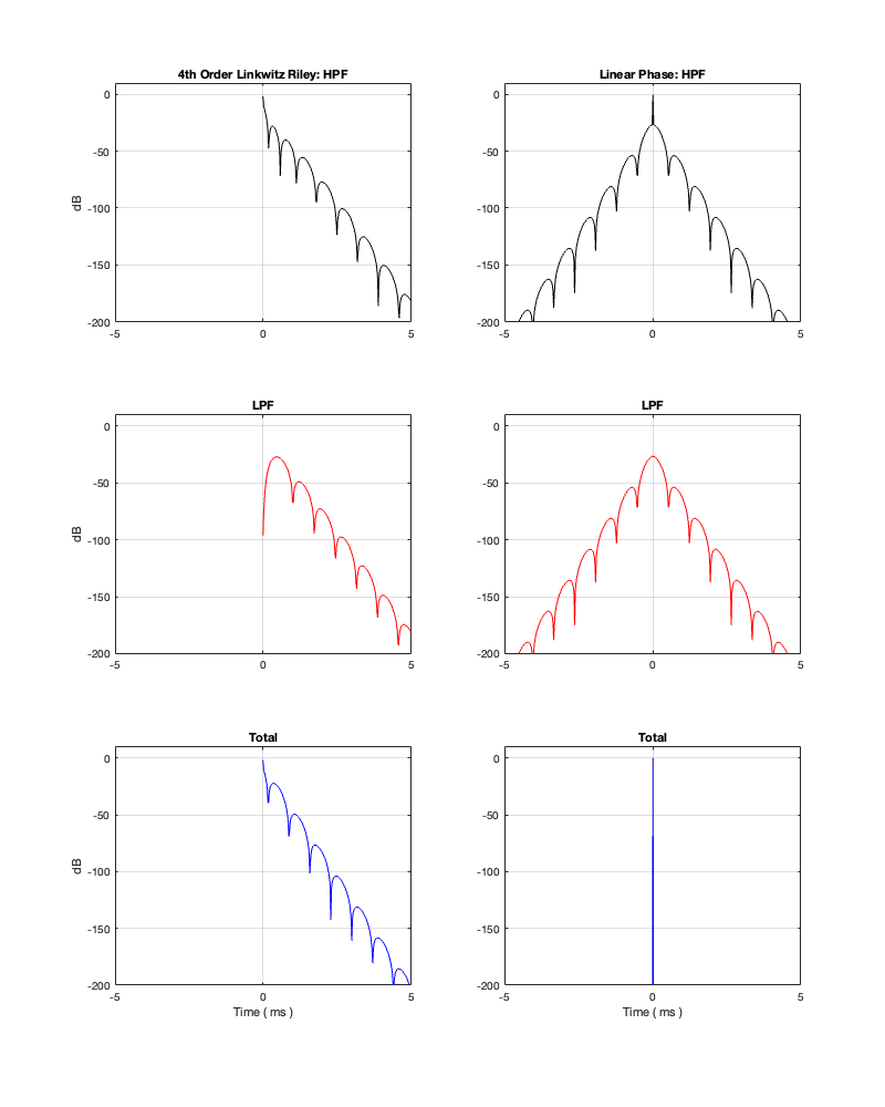
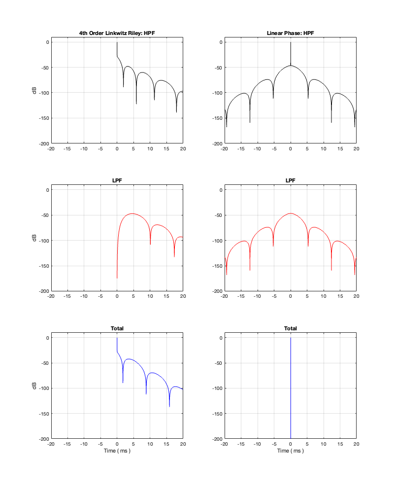
How late? That’s up to you, since it’s a combination of the filter’s frequency and how accurate and precise you want the filter to be. One way to consider this is to look at the plots in Figure 12.4 on a decibel scale. This is shown in Figure 12.5.
Figure 12.5: the same impulse responses shown in Figure 12.4, on a decibel scale.
Let’s say, for example, that you have this crossover at 1 kHz and you want to have an impulse response that is accurate down to -100 dB. Looking at HPF and LPF impulse responses for the linear phase crossover, we can see that they drop below -100 dB at about ± 2.4 ms. This means that, if you decide that your threshold of acceptability is about -100 dB (which is pretty good…) then, for a 1 kHz linear phase crossover, you’ll have to include a 2.4 ms delay in your signal path to implement it.
Of course, if you are more picky – say, you want to go down to -200 dB instead, then you’ll have to wait about 4.8 ms (check where the red and black lines get 200 dB down on the left side of the plots.
Notice that I said above that this amount of time – the delay (or as we normally call it: the loudspeakers input-output latency) is also dependent on the frequency of the filters.
So, let’s look at the same plots for a crossover that is one decade lower: at 100 Hz.
Figure 12.6
Figure 12.7
Figure 12.8
Figures 12.6 to 12.8 show the same plots for at 100 Hz crossover. HOWEVER: notice that the scale of the x-axis has changed to ±20 ms instead of ±5 ms. Also note that, despite me extending that scale by a factor of 4, it’s still not enough to get down 200 dB for the linear phase filters.
You can see there (looking at the red curve on the right of Figure 12.8) that, if you’re going to set -100 dB as your threshold, then you will have to have a latency of about 14 or 15 ms to implement it as a linear phase crossover. (Similar to the 1 kHz version, if you want to go down 200 dB, you’ll need to double this to 28 to 30 ms, which is starting to get close to the acceptable limits for lip-synch with video.)
In the next posting, we’ll look what happens to the magnitude and phase responses if you shorten these impulse responses using a technique called “windowing”.
However, I am NOT going to talk about audibility of a linear phase vs a minimum phase strategy. There are people who love to bang on about ringing and pre-ringing and whether you can hear the “ramp in” of the linear phase filters, or whether the “long” decay time of the minimum phase filters are audible. The best way to stay out of this fight is to not comment on it. If you want to decide whether you can hear these things or not, then you should implement them and have a listen. I can’t tell you what you can or cannot hear. However, if you DO decide to try implementing these for a listening test, make sure that you do it right, that:
the only difference in the crossovers is what you think it is (If not, you’re not comparing the crossover types in isolation), and
you are running a blind test (if not you can’t trust your own opinion).
you cannot just stick a crossover in front of some loudspeaker drivers and expect the total system to behave
the on-axis response and the power response of a loudspeaker are related to each other
the power response is also very dependent on the directivity characteristics of the individual drivers and they way they interact (including the crossover’s effects) in three-dimensional space
if you fix something for the on-axis response, you might do damage to the power response
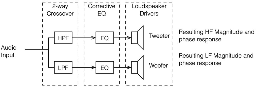
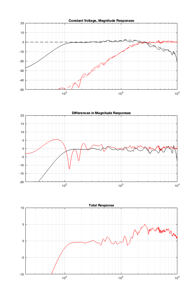
Now we’re going to do something that I didn’t do in the previous posting. I’ll use the crossover responses as a TARGET for the total response of the crossover + driver outputs.
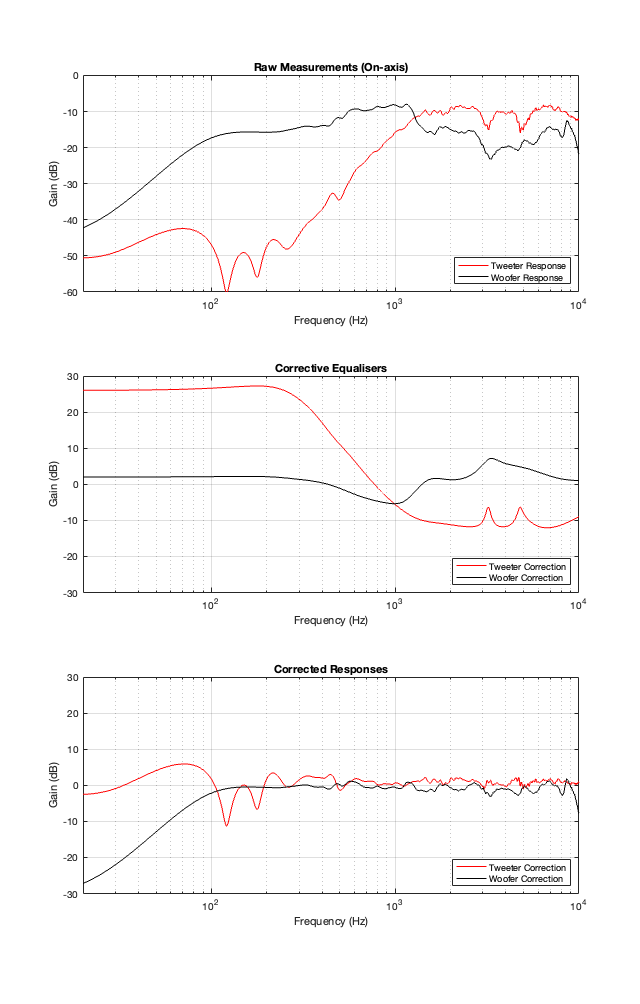
Figure 11.1. Feel free to ignore the response of the tweeter (in red) below about 300 Hz. That’s probably just an artefact of the way it was measured.
The top plot in Figure 11.1 shows the magnitude responses of the raw measurements of the tweeter and woofer that we looked at in Part 10. I then used these measurements to quickly make some agressive equalisation curves to force them to be flat-ish. These two equalisation filters are shown in the middle plot of Figure 11.1. Each of these is the product of a LOT of filters that I put in to result in the curves of the combined total responses that you see in the bottom of Figure 11.1.
In theory, if you play the tweeter and woofer through their respective equalisers, you will be able to measure the magnitude responses that you see there in the bottom of Figure 11.1. Of course, a 1″ tweeter can play a 20 Hz sine tone, it just can’t do it very loudly. So, this is NOT the solution to making a loudspeaker. This is just for illustrative purposes.
Figure 11.2
If I then apply our crossovers to these equalised loudspeaker drivers as shown in the signal flow above, I get the plots below.
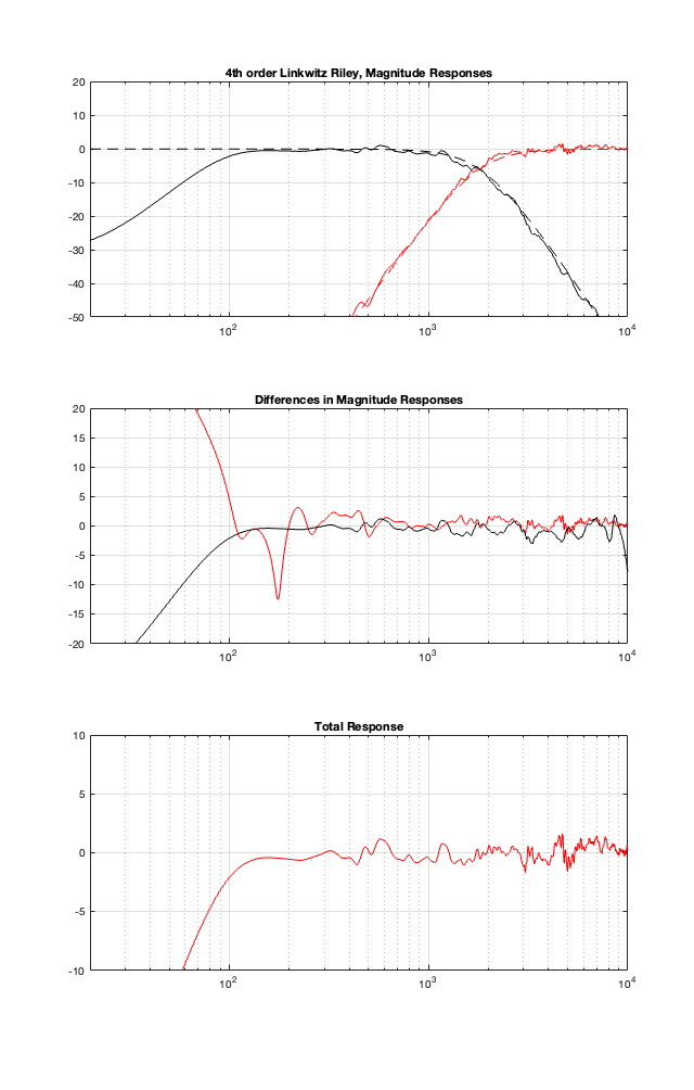
4th order Linkwitz Riley
Figure 11.3. Compare these to the plots in Part 9, Figure 9.5, but it’s important to notice that this last scale is 20 dB (-10 to +10) whereas the scale in Part 5 is 70 dB (-50 to +20)
The top plot of Figure 11.3 shows the target magnitude responses of a 4th-order Linkwitz Riley crossover as the dotted lines. The solid lines show the measured outputs of the woofer and tweeter, including the corrective equalisation.
The middle plot shows the differences in what I want the crossover to do, and what the actual responses are at the outputs of the loudspeaker drivers. Again, in a perfect world, these would be two flat lines, sitting on 0 dB at all frequencies.
The bottom plot is the resulting on-axis response of the loudspeaker, combining the two outputs. Notice how much flatter it is than the one we had in Part 10. (the scale of this plot is much tighter than it was in the previous posting…)
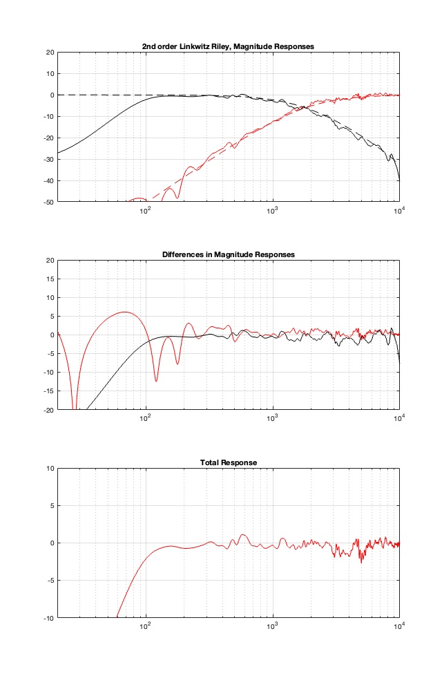
2nd Order Linkwitz Riley
Figure 11.4. Compare these to the plots in Part 9, Figure 9.6, but it’s important to notice that this last scale is 20 dB (-10 to +10) whereas the scale in Part 5 is 70 dB (-50 to +20)
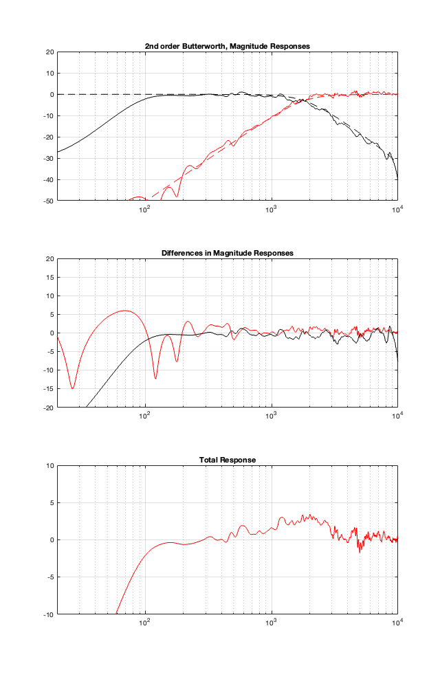
2nd order Butterworth
Figure 11.5. Compare these to the plots in Part 9, Figure 9.7, but it’s important to notice that this last scale is 20 dB (-10 to +10) whereas the scale in Part 5 is 70 dB (-50 to +20)
One comment here. Notice the +3 dB bump around the 1.8 kHz crossover, just like we would expect from a 2nd-order Butterworth crossover.
Constant Voltage
Figure 11.6. Compare these to the plots in Part 9, Figure 9.8, but it’s important to notice that this last scale is 20 dB (-10 to +10) whereas the scale in Part 5 is 70 dB (-50 to +20)
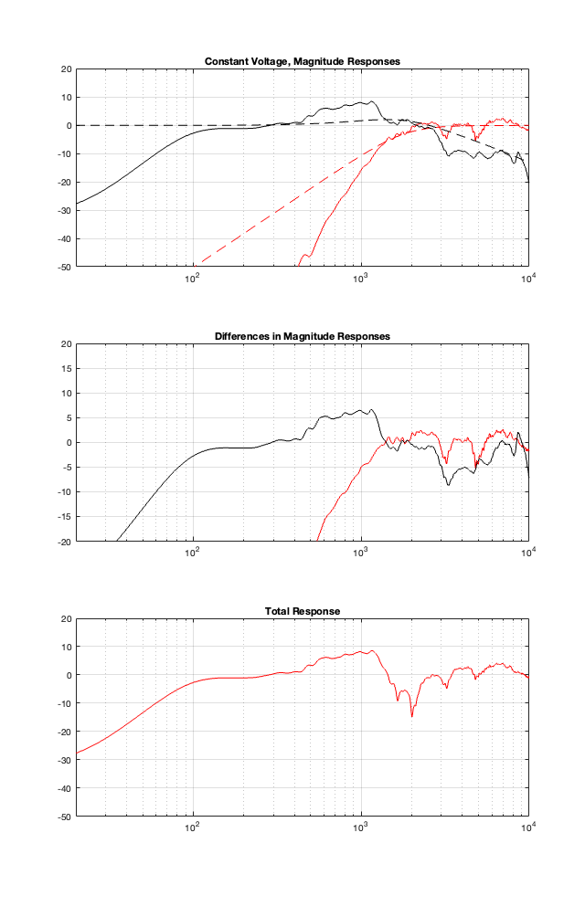
This one is interesting, but not surprising. You can see here that there is an unexpected high-shelving characteristic here in the total response. The reason for this is the combination of a number of things:
the corrective EQ that I made was a bit quick-and-dirty, only using minimum phase filters
a constant voltage crossover is very sensitive to phase variations in the two signal paths. If they don’t behave as one would expect (and they don’t in this loudspeaker because of my corrective EQ) then things get a little weird.
Finally, take a look at the dotted lines. You can see there that the woofer has a lot of contribution in the high end. This combines with the previous point to make the total a little unpredictable.
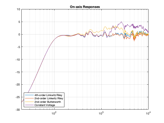
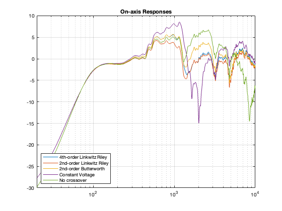
Just for comparison, here are the on-axis responses plotted in one figure.
Figure 11.7
Power Responses
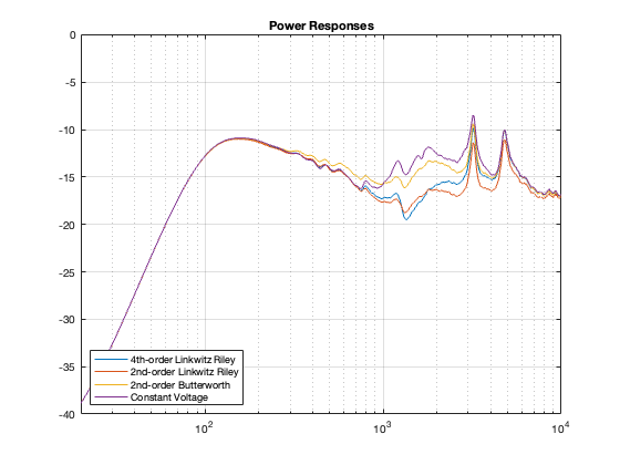
Finally, you might ask what the power responses look like for these loudspeakers. They’re shown below in Figure 11.8
Figure 11.8. Compare this to the Power Response plots in Figure 10.1 in Part 10.
You might be surprised by the fact that, although most of our on-axis magnitude responses look pretty flat, the Power Responses are not nice, straight lines with a general downward slope. In fact, they have some pretty ugly peaks there. Why? This is because I did my equalisation based on only one on-axis measurement. So, by focusing all of my attention on that one point in space, I sacrificed the response of the spherical radiation. If we were making a loudspeaker for an anechoic chamber, and we had only one chair and no friends, this would be fine. However, this would NOT be a good solution for a loudspeaker that’s designed for a real room that has some reflections.
On the other hand, there is one interesting thing that’s worth noting in those plots.
The downward slope from about 150 Hz to about 1 kHz is the result of the woofer “beaming” as the frequency increases. The total power in the three-dimensional radiation of the loudspeaker drops because there’s less and less energy radiating backwards – and therefore less and less total power.
Above this, the power responses increase again because we’re moving into the tweeter, which is more omnidirectional in its low end.
It’s also interesting to compare this plot to Figure 10.1 in Part 10. Notice that the transition in the slope just above 1 kHz has disappeared. This is because the responses of the two drivers have been cleaned up by the individual equalisation.
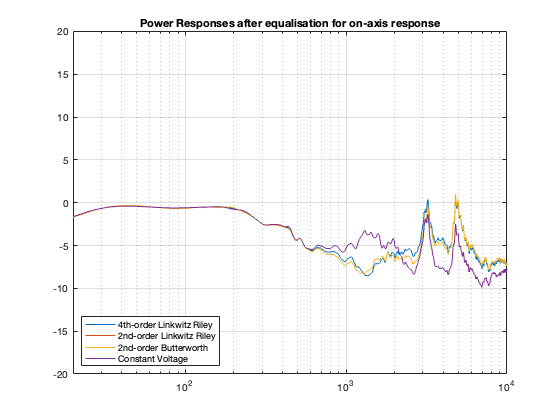
One last thing to notice is the that the similarity between the curves in this plot is a lot like the curves in Figure 10.3 in the previous posting. This is because, in both cases, I’m doing some kind of correction for the on-axis response. In Part 10, I put in a correction for the on-axis response of the entire loudspeaker after the tweeter and woofer outputs were summed. In this posting, I corrected for the individual loudspeakers’ on-axis responses before summing them. Although the two methods are different, the end results are similar to each other. Another way to think of this is that correcting for the on-axis response makes the power responses of the different crossover types more similar to each other.
Just for completeness, Figure 11.9 shows the Power Responses if I were to apply a “dumb” filter that REALLY flattens the on-axis response after all of this. You shouldn’t need to do this, since the individual drivers were flattened in advance. Compare this one to Figure 10.3 in Part 10.
Figure 11.9.
N.B. About a week after I made this posting, I found an error in my Matlab code that calculated the plots. They’ve now been updated to the correct curves. The general conclusions listed in the text haven’t changed, but some of the little details have.
Extra note for the sake of transparency
Figure 11.9 was made using a method that is about as stupid and lazy as I could have possibly done. For each crossover type, all I did was to subtract the values shown in the plot in Figure 11.7 from those in Figure 11.8. This is probably not the way that you would implement a “flattening” filter in real life, but it is similar to the old-fashioned strategy used by systems that blindly make an FIR filter based on a single measurement.
In this posting, we’ll do something similar to the analyses from Part 7. In that one, we
took two point-source theoretically perfect loudspeaker drivers (which means that they have the same magnitude response in all directions in 3D space), (pretending that they were a tweeter and a woofer in a non-existent cabinet)
filtered each of their inputs using a crossover network
separated them by some distance
measured them in a bunch of places on a sphere surrounding the non-existent cabinet
found the total magnitude response of the system when measured all around on that sphere, which is called the loudspeaker’s Power Response.
Now, we do that again, but we will include the real loudspeaker drivers’ measurements in that three-dimensional world. In this case, we still have the 1″ tweeter and the 6″ woofer in a sealed cabinet. Those two loudspeaker drivers were individually measured at 130 points around them on that sphere that I showed in Part 7.
I then take each of those 130 measurements for each driver, filter them using the crossover, and add the two outputs together, which gives me the magnitude response of the entire loudspeaker with two drivers for each individual location. We then add the 130 measurements to find a total combined response which is the Power Response of the two-way loudspeaker with two real loudspeaker drivers in a real cabinet, with the 5 different crossover types that we’ve been talking about.
Note that I have NOT done what I said I SHOULD do at the end of part 9. I have just been dumb and stuck the crossovers in front of the loudspeaker drivers without thinking about modifying the filters to compensate for the drivers’ characteristics.
The five resulting power responses are shown in Figure 10.1.
Figure 10.1
The first thing to notice is that there is a roll-off in the low end. This is the natural response of the woofer that we saw in Part 9.
The second thing that you’ll notice is the general downward-slope in the top octave of the plot, starting at about 7 kHz and having a generally decreasing magnitude the higher you go in frequency. This is the result of “beaming”. Since the two loudspeaker drivers, generally, have less and less high-frequency output as you move off-axis, then this appears as less total output from the system on that sphere. If the two loudspeakers were omnidirectional, then the power response would be a horizontal line. The more directional the drivers, the steeper the downward slope of this plot.
The last thing that’s easy to see in this plot is the transition between the woofer and the tweeter. It appears as that steep slope just above 1 kHz. Remember that I put the crossover at 1.8 kHz – so the slope doesn’t sit right on the crossover frequency. But it’s easy to see that something is happening to the directivity of the loudspeaker in that area.
Now remember back to Part 7, where we did a little trick where we made an assumption that a person building or installing a loudspeaker would measured its on-axis response, and then put in an equaliser to flatten this measured response.
In the old days, you would do this “by eye” using something like a graphic or a parametric equaliser. But nowadays, we have fancy tools that can do measurements and create complicated FIR filters that do whatever we want. This means that we can REALLY screw things up with the precision of a surgical scalpel…
So, let’s be dumb and do the same thing again. We’ll take the on-axis responses of the loudspeaker with the different crossovers (we already saw these in Part 9, but here they are again, shown in Figure 10.2), and we’ll make five “perfect” equalisers that make each of these five responses perfectly flat.
Figure 10.2
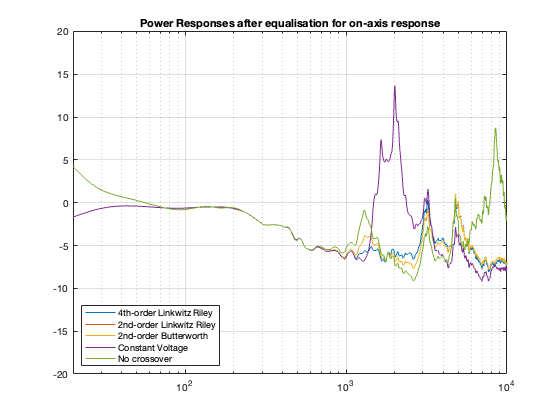
After applying each of these customised filters that make our on-axis measurement look like a laser beam, we should probably check what happened to the power responses. They’re shown below in Figure 10.3.
Figure 10.3
As you can see there, the low frequency response flattens out. This is because we’re really boosting the bass (to fix the on-axis measurement) and this loudspeaker happens to be fairly omnidirectional below about 200 Hz.
You can also see that I was REALLY dumb when I made those equalisation filters. For example, the notch in the on-axis response of the Constant Voltage caused me to make a horrendous peak that results in a really nice-looking plot at one on-axis point in space, but completely messes up the response of the loudspeaker in almost all other directions, resulting in that giant 15 dB peak around 2 kHz (remember that our crossover frequency is in this region…). I also wound up pushing up the low end by something like 30 dB, which is nuts.
The moral of this story is “don’t fix the on-axis response without considering the power response”. OR “just because it looks flat doesn’t mean that it’ll sound good.” On the other hand, notice that, after equalisation, most of the other curves look pretty similar-ish which means that maybe doing some intelligent equalisation for the on-axis response isn’t necessarily a bad idea.
Remember, however, that we’re still only looking at the loudspeaker in infinite space. There’s no room “singing along” with this loudspeaker… but the topic of room compensation is for another time…
N.B. About a week after I made this posting, I found an error in my Matlab code that calculated the plots. They’ve now been updated to the correct curves. The conclusions listed in the text haven’t changed, but some of the little details have.
Extra note for the sake of transparency
Figure 10.3 was made using a method that is about as stupid and lazy as I could have possibly done. For each crossover type, all I did was to subtract the values shown in the plot in Figure 10.2 from those in Figure 10.1. This is probably not the way that you would implement a “flattening” filter in real life, but it is similar to the old-fashioned strategy used by systems that blindly make an FIR filter based on a single measurement.
Up to now, we’ve either assumed that we don’t have any loudspeaker drivers in the chain (Parts 1 to 5 inclusive) or that our loudspeaker drivers are “perfect” point sources (Parts 6 to 8 inclusive). This means that, so far, our nice, perfect world has used a model that looks a little like Figure 9.1
Figure 9.1.
Now, we start getting a little closer to reality by adding some actual loudspeaker drivers to the outputs of the crossover. Going forward, I’m using the actual measurements of a real 1″ tweeter and a real 6″ woofer in a real sealed cabinet. So, now, instead of just looking at the magnitude and phase responses of the crossover’s outputs, we’re looking at the responses of the outputs of the drivers, as shown in Figure 9.2. Another way to think of this is that we have extra filters (the drivers’ responses, which are different in different directions) in addition to the filters in the crossover.
Figure 9.2
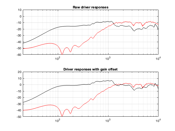
The problem with real loudspeakers is that they aren’t perfect, so let’s start by looking at their responses on-axis. These are shown in Figure 9.3
Figure 9.3.
The top plot of Figure 9.3 shows the on-axis magnitude responses of the loudspeaker drivers in the cabinet without any filtering. The bottom plot shows the same responses, with gain offsets to match them at an arbitrary crossover frequency of 1800 Hz.
4th Order Linkwitz Reily
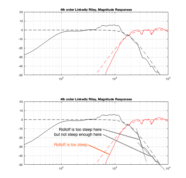
If I apply filtering using a 4th-order Linkwitz Reily crossover, and then send its outputs to a tweeter and a woofer, the resulting magnitude responses of the two drivers, when measured on-axis to the cabinet will look like the top plots in Figure 9.4, below.
I’ve duplicated the plot in the bottom half of the figure, and added some comments. Notice that the responses of the actual loudspeaker outputs, including the crossover filter, do NOT look like the theoretical responses of the crossover itself (shown as dotted lines). On-axis, the tweeter has a natural high-pass characteristic (seen in Figure 9.3) that, when combined with the high pass filter in the crossover, results in a slope that’s too steep.
The woofer’s rolloff is weird in that its contribution makes the low pass filter too steep at the start of the rolloff, and then not steep enough as you get a little higher in frequency. If you look back to Figure 9.3, this can be seen as the dip in the response that produces the “bowl” shape from roughly 1 kHz to 8 kHz.
Figure 9.4.
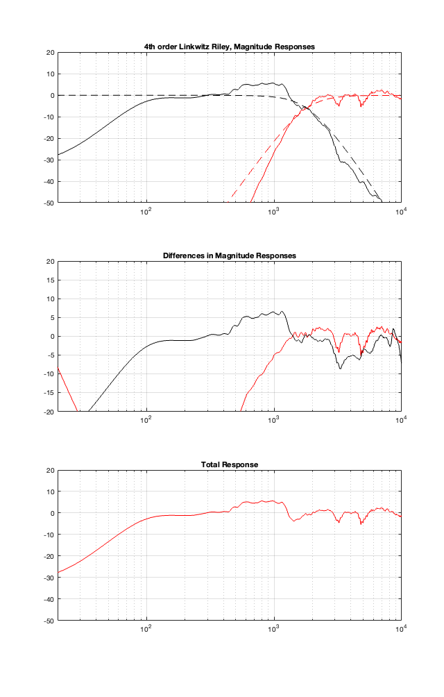
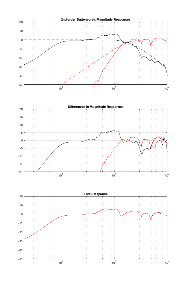
This means that, if we ignore the natural on-axis magnitude and phase responses of the loudspeaker drivers, and just slap a crossover in front of them, the resulting total response won’t be as pretty as we would expect. This is shown in the bottom plot in Figure 9.5.
The plots shown in the middle of Figure 9.5 are the difference between what we WANT the crossover to be (the dotted lines in the top plot) and the ACTUAL total resulting magnitude response at the outputs of the drivers (the solid lined in the top plot). In other words, these curves show the vertical distance between the solid and dotted lines in the top plot. If the drivers had perfectly flat magnitude responses, then these two lines would be flat, and they would sit on the 0 dB line.
Figure 9.5.
You might say that the Total Response in Figure 9.5 looks pretty good. I would disagree. An on-axis in-band magnitude response of about ±5 dB is pretty terrible if your goal is a flat on-axis response. If this is not your goal, then I have no opinion.
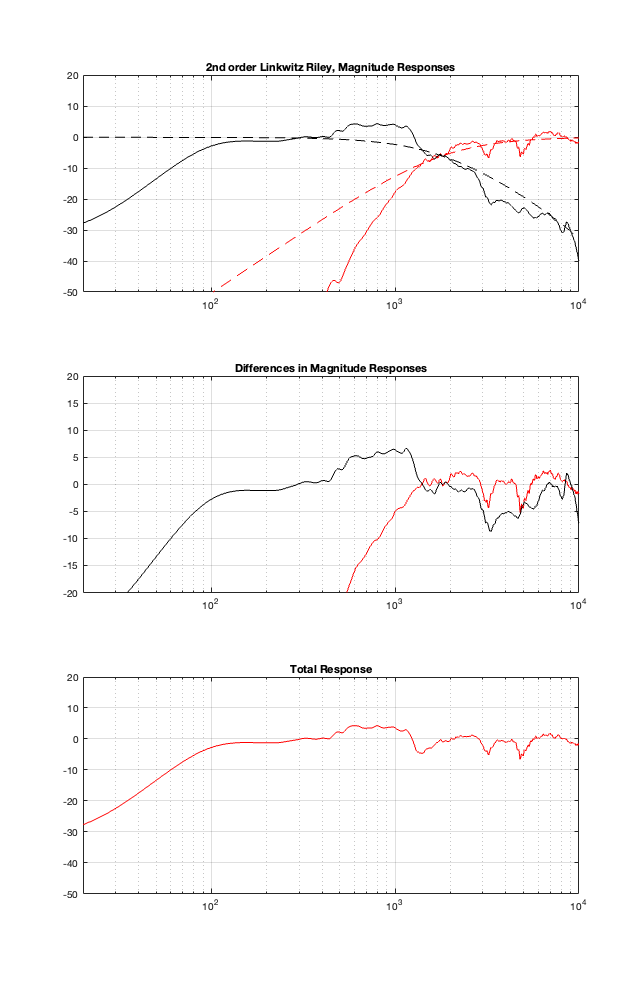
Now I’ll just throw in the same plots for the different crossover types, implementing the crossover with the assumption that the loudspeaker drivers are perfect, and then doing the analysis including the actual responses of the drivers.
2nd order Linkwitz Reily
Figure 9.6
2nd order Butterworth
Figure 9.7
Constant Voltage
Figure 9.8
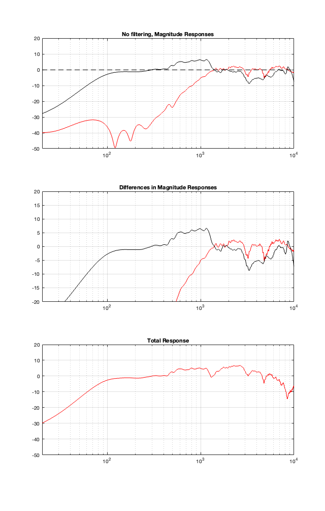
No Crossover
Figure 9.9
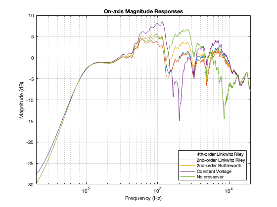
Comparison
Figure 9.10. The five total responses of the crossover types from the plots above.
I’ll let you draw your own conclusions about the results of these plots. I will highlight one thing: remember that the theoretical combined magnitude responses of the 4th order Linkwitz Riley and the Constant Voltage crossovers are both flat. But compare their Total Responses in the plots above. Notice that they are very different from each other. This is, in part, because the phase responses of the two signal paths are modified by the driver’s behaviours, which means that they don’t add as nicely as we would like.
The moral of the story this time is: you can’t ignore the natural response of the drivers when you’re designing your crossover. This means that we will need to change our filters to ensure that the TOTAL response of the filter PLUS the driver results in the response that we want. The design of the crossover MUST include the responses of the drivers to ensure that it behaves as we wish.
But, so far, we have only considered this at one point in space, directly in front of the loudspeaker. In the next posting, we’ll come back to looking at the total power response. Things are about to get ugly…
This will be a short posting with very little new information. I’m just starting to put some of the Lego blocks together to make it easier later on.
For this posting, I’ve taken two different pieces of information that you already have, and put them together.
2nd order Butterworth
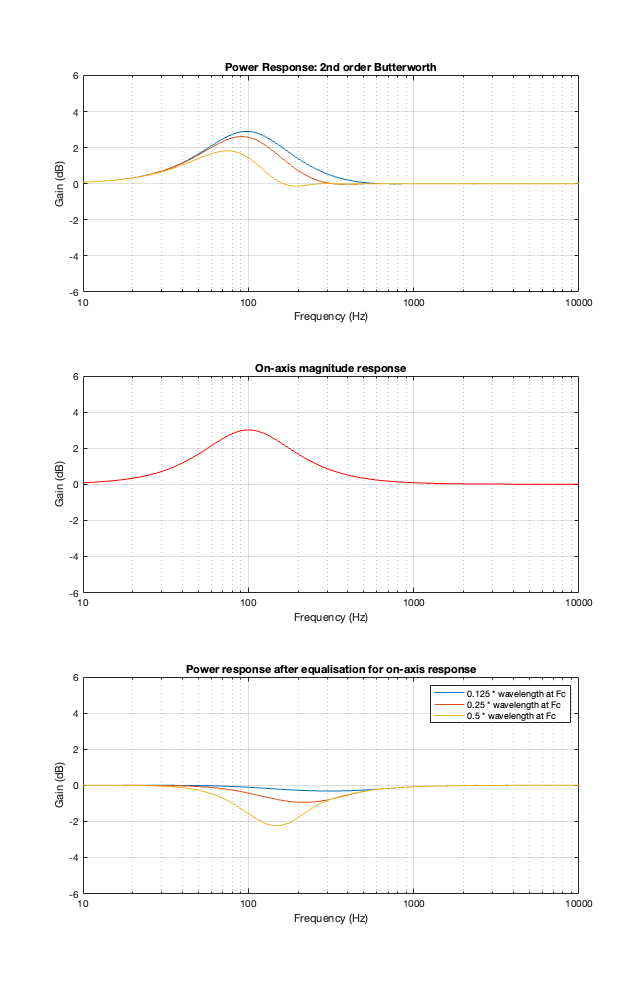
Take a look at Figure 8.1 below, which shows information related to a 2nd order Butterworth crossover at 100 Hz.
The top plot shows the power responses, explained in Part 7.
The middle plot shows the on-axis magnitude response, which will be the same regardless of the separation between the loudspeaker drivers because I’m assuming that they’re perfect point-sources.
IF you built such a loudspeaker, then chances are that you would put in an equaliser at the input of your loudspeaker to make the on-axis response flat instead of having that bump. That equaliser would, in turn effect the entire power response. So, the bottom plots show the power responses of the loudspeaker (with three different driver separations) AFTER you’ve applied the equalisation to correct for the on-axis magnitude response.
In other words, the top plots MINUS the middle red plot equals the bottom plots
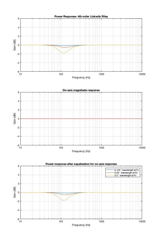
4th-order Linkwitz Riley
The 4th-order Linkwitz Riley’s power response does not change because its on-axis response is flat, so there’s nothing to correct.
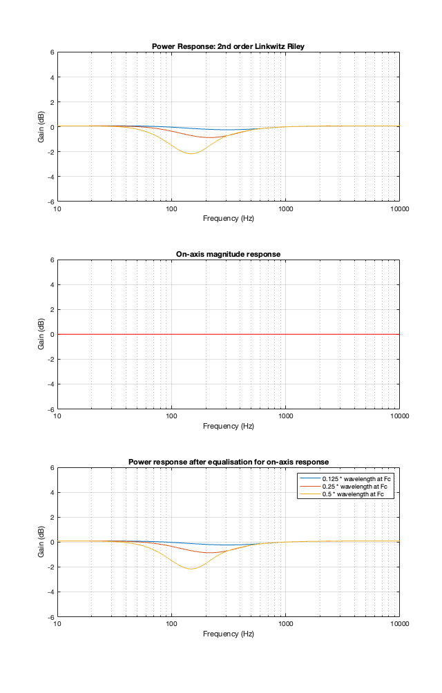
2nd-order Linkwitz Riley
The 2nd-order Linkwitz Riley’s power response does not change because its on-axis response is flat, so there’s nothing to correct.
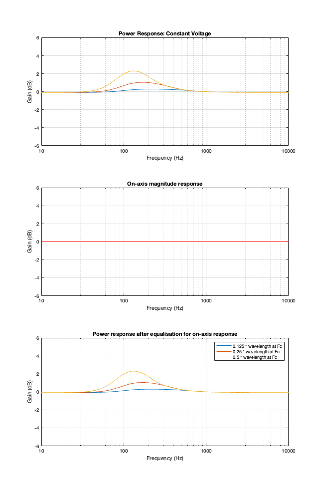
Constant Velocity
The Constant Velocity’s power response does not change because its on-axis response is flat, so there’s nothing to correct.
Like I said: there’s no new information here. It’s just a reminder that, if you add equalisation for your on-axis response (whether this is part of your loudspeaker-building process or your installation in the listening room), you will also have a subsequent on the power response. Since the equalisation is applied to the loudspeaker’s input, the on-axis and power responses are locked together. Change one, and you change them both.