I’ve started working with a number of my colleagues on a series of videos for internal training at Bang & Olufsen. They were kind enough to make some of these videos publicly available.
This video explains why loudspeaker drivers are typically put in enclosures (boxes), the three types of enclosures that we use (sealed, ported, and passive radiators), and the differences in impact that these enclosure types have on the loudspeaker’s behaviour.
I’ve started working with a number of my colleagues on a series of videos for internal training at Bang & Olufsen. They were kind enough to make some of these videos publicly available.
This video explains the various components inside a typical loudspeaker driver.
It’s been a long time (about 11 years or so…) since I wrote Part 1 in this “series”, so it’s about time that I came out with a Part 2. This one is about the ‘Maximum Sound Pressure Level (SPL)’ and the ‘Bass Capability’ values that are shown for each loudspeaker model on the Bang & Olufsen website.
Before I explain either of those numbers, we need to discuss the fact that B&O loudspeakers are fully-active. This means that all the signal processing, including simple things like the volume control and more complicated things like filtering and crossovers for the loudspeaker drivers happen in a digital signal processing (DSP) chain before the amplifiers, which are individually connected to the loudspeaker drivers. (In other words, if you see a woofer and a tweeter, then there are two amplifiers inside the loudspeaker, one for each.)
That DSP chain includes even more complicated features that help to protect the loudspeaker from abuse. This means that, even if you’re playing a signal that’s been mastered at a high level, and you’ve cranked up the volume control, the processor prevents things like:
letting the loudspeaker drivers exceed their maximum excursions
letting the amplifiers go beyond their voltage or current capabilities
letting the power supply try to deliver more current than it can to the entire system
letting the loudspeaker’s internal components get so hot that things start to melt.
(None of this means that it’s impossible to break the loudspeaker. It just means that you’d have to try a lot harder than you would with a lot of other companies’ loudspeakers.)
One important side-effect of all of those protection algorithms is that, when you play a loud signal at maximum volume, the loudspeaker will be constantly trying to protect itself. Therefore its maximum output level will vary over time, depending on the signal you’re playing and things like the temperatures of its various individual components.
This, in turn, makes it difficult to state what the “Maximum Sound Pressure Level” will be, since it will change over time with different conditions.
On the other hand, it’s necessary to give a number that states the maximum Sound Pressure Level of each loudspeaker for lots of reasons. It’s also necessary that we use the same procedure to do the measurement so that the values can be compared from loudspeaker to loudspeaker.
The method
So, how do we balance these two things? The answer is to make the measurement short enough that we show the maximum output of the loudspeakers when it’s hitting its limits without being affected by a build-up of heat. This can give you an idea of how loud a short-term signal (like the punch of a kick drum or a snare drum hit) can play: the Maximum SPL. Whatever that number is, the loudspeaker definitely can’t play louder than it (since the amplifier can’t deliver more current and the loudspeaker drivers can’t move in and out any further) but that doesn’t necessarily mean it can play at that level continuously.
The way we measure both the Maximum SPL and the Bass Capability is by placing a microphone 1 m in front of the loudspeaker, and then putting in a short ‘burst’ of 5 periods of a sinusoidal tone at a given frequency. The sound pressure level of the output is measured at the microphone’s position, we wait long enough for everything to cool down, the level of the incoming signal is increased, and then we do the measurement again. This is repeated until the output signal’s level is being automatically reduced by the loudspeaker’s protection algorithms by a pre-determined amount (-6 dB).
If we were a company that made passive loudspeakers, a normal way to do this would be to increase the level until we reached a pre-determined level of total harmonic distortion (say, 10% or 20% THD, for example). However, this won’t work for a B&O loudspeaker because the protection algorithms probably won’t allow the product to distort enough to have a usable threshold.
What’s the difference?
Generally, the method of measuring both the Maximum SPL and the Bass Capability values are the same. The only difference is the range of frequencies that are used for each.
The Bass Capability shows the maximum SPL of the loudspeaker when the input signal is a 50 Hz sinusoidal wave.*
The Maximum Sound Pressure Level is an average of the maximum SPL of the loudspeaker when it is measured using a number of sinusoidal signals ranging from 200 Hz to 2 kHz. Each frequency is measured individually, and the resulting maxima are averaged to produce a single value. (If you’re read Part 1, then the frequency range of this measurement will look familiar.)
How does this correspond to real life?
This is a difficult question to answer, since the measurement is done on-axis to (or ‘directly in front of’) the loudspeaker in the measurement room. This measurement room is different from a ‘normal’ living room, where more of the total power of the loudspeaker that’s radiated in all three dimensions is reflected back to the listening position. This is the reason why some companies list the maximum output level of their loudspeakers with two numbers: one in a ‘free field’ (a room or ‘field’ that is ‘free’ of reflections) and the other in a ‘listening room’ (which may or may not be like your listening room). You’ll probably see that the ‘listening room’ SPL is higher than the ‘free field’ SPL because the room is reflecting more energy back to the measurement microphone, if nothing else…
In other words ‘results may vary’. So, the maximum SPL of a loudspeaker in your living room may not be the same as the Maximum SPL that B&O lists on its website. Time frames are different, signals are different, and rooms are different: and all of these have significant effects on the result.
What happens when I have more than one loudspeaker?
Generally speaking, if your loudspeakers are reasonably far apart, then you can use a simple rule to calculate the maximum SPL if you add more loudspeakers.
+ 3 dB per doubling
In other words, if you have a loudspeaker that can hit 100 dB SPL, and you add a second loudspeaker, then you’ll hit 103 dB SPL. If you then add two more loudspeaker (another doubling of the total number) you’ll hit 106 dB SPL.
This rule is based on a number of assumptions:
the loudspeakers are all the same type
the loudspeakers are in the same room, but fairly far apart
the loudspeakers are all playing their maximum output levels at the same time
I’m ignoring room modes, which might make things louder or quieter, depending on the frequency that you’re playing, the placements of the loudspeakers, and the location of the listening position
we’re ignoring other protection algorithms like thermal protection
The reason that this rule is a basic one: we’re assuming that every time you double the number of speakers, you double the total power at the listening position (which is a reasonable assumption if the list of assumptions above are true). Two times the acoustic power is the same as an increase of +3 dB SPL (because 10 log10(2) = 3).
If, however, the frequency was very low, and the loudspeakers were very close together, and they were playing exactly the same signals at exactly the same time, you might make the argument that you can say that there is a +6 dB increase for every doubling of loudspeakers, because it’s their amplitudes (and not their acoustic powers) that are added.
Neither of these two basic assumptions is correct, and so the real number is probably between +3 and +6 dB per doubling of loudspeakers, and it will be different for different frequency bands and different loudspeaker separations. However, it’s best to err on the safe side.
One last thing
This should help to explain why, when you compare the Bass Capabilities and the Maximum Sound Pressure Levels of different loudspeakers, the former has much bigger differences than the latter.
For example:
Beosound Explore
< difference >
Beolab 50
Max SPL @ 1 m
91 dB SPL
26 dB
117 dB SPL
Bass capability
59 dB SPL
52 dB
111 dB SPL
The table above shows a direct comparison of two VERY different loudspeaker models using data taken directly from bang-olufsen.com on 2025 04 01. I’ve converted the numbers for the Beolab 50 to a ‘per loudspeaker’ instead of ‘per pair’ by subtracting 3 dB from the published numbers.
As you can see there:
the difference in Bass Capability between a Beosound Explore and a Beolab 50 is (111-59) = 52 dB
the difference in Max SPL between a Beosound Explore and a Beolab 50 is (117-91) = 26 dB
Speaking VERY generally, the difference in Max SPL values is less than the difference in Bass Capabilities because the difference in size and power of the drivers producing the midrange frequency band of the two loudspeakers is smaller than the difference in size and power of the woofers. In other words, there is a difference between the different differences. (I think that I got that right…)
* To get the Bass Capability measurement, it looks like I said that we do the measurement of a single 50 Hz sinusoidal tone. This isn’t really true. We do a number of measurements at different frequencies ranging from 20 Hz to 100 Hz and then calculate the equivalent value for a 50 Hz tone using some averaging.
If the loudspeaker is comprised of a single low-frequency driver in a closed cabinet, then the resulting number would be the same as if we just measured using a 50 Hz tone. However, if the loudspeaker is ported or has a passive driver with a resonant frequency in the 20 – 100 Hz range, then this method will probably produce a slightly different number than measuring only with a 50 Hz tone.
In Part 2, I showed the raw magnitude response results of three pairs of headphones measured on three different systems, each done 5 times. However, when you plot magnitude responses on a scale with 80 dB like I did there, it’s difficult to see what’s going on.
Differences in measurements relative to average
One way to get around this issue is to ignore the raw measurement and look at the differences between them, which is what we’ll do here. This allows us to “zoom in” on the variations in the measurements, at the cost of knowing what the general overall responses are.
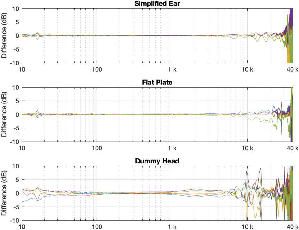
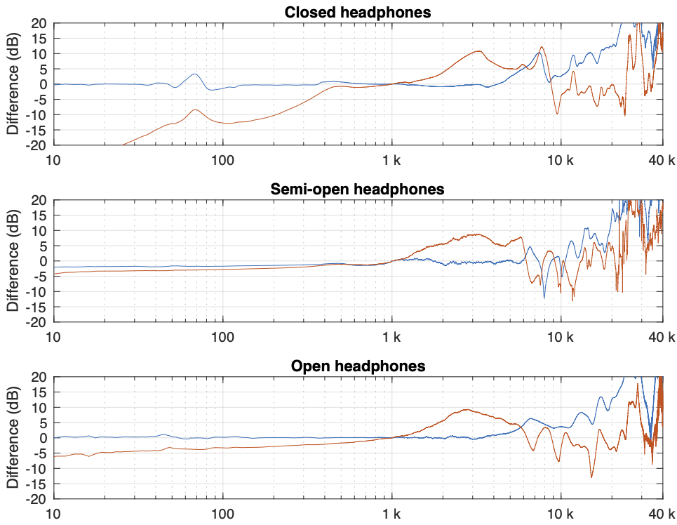
Figure 1 in Part 2 showed the 5 x 3 sets of raw magnitude responses of the open headphones. I then take each set of 5 measurements (remember that these 5 measurements were done by removing the headphones and re-setting them each time on the measurement rig) and find their average response. Then I plot the difference between each of the 5 measurements and that average, and this is done for each of the three measurement systems, as shown below in Figure 1.
Figure 1: Open headphones: The difference between each of the 5 measurements done on each system and the mean (average) of those 5 measurements.
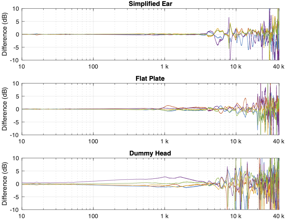
Figure 2: Semi-open headphones: The difference between each of the 5 measurements done on each system and the mean (average) of those 5 measurements.
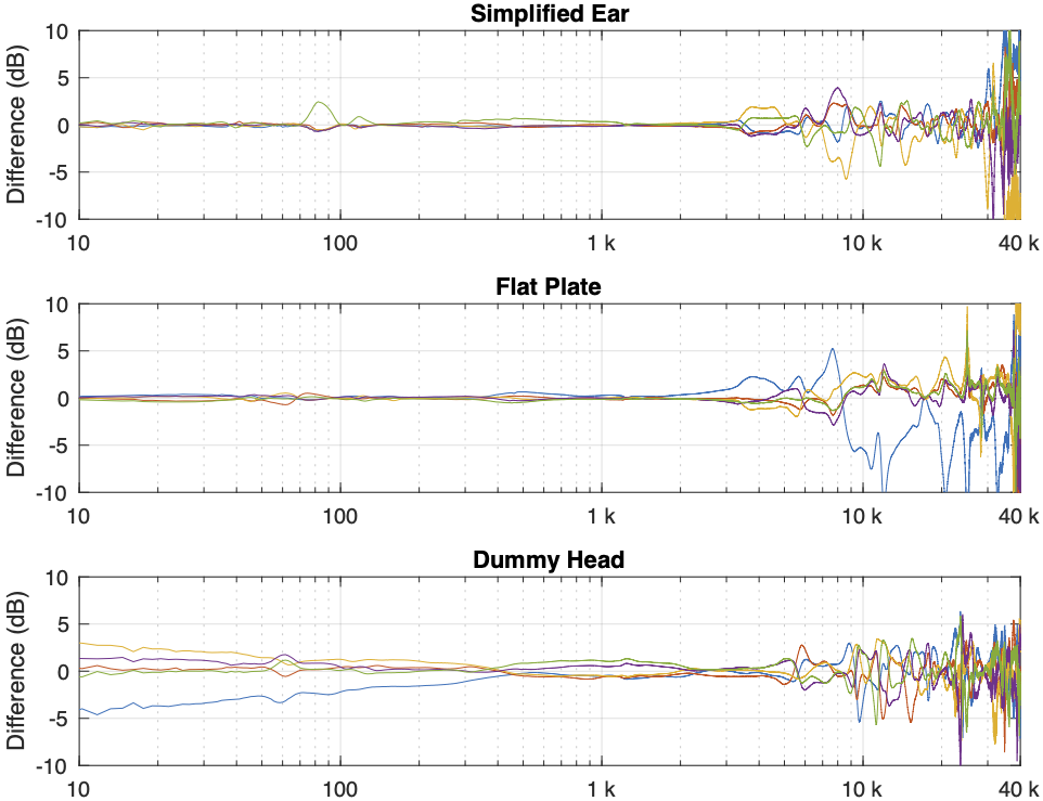
Figure 3: Closed headphones: The difference between each of the 5 measurements done on each system and the mean (average) of those 5 measurements.
Some of the things that were intuitively visible in the plots in Part 2 are now obvious:
There is a huge change in the measured magnitude response in the high frequency bands, even when the pair of headphones and the measurement rig are the same. This is the result of small changes in the physical position of the headphones on the rig, as well as changes in the clamping force (modified by moving the headband extension). I intentionally made both of these “errors” to show the problem. Notice that the differences here are greater than ±10 dB, which is a LOT.
Overall, the differences between the measurements on the dummy head are bigger and have a lower frequency range than for the other two systems. This is mostly due to two things:
because the dummy head has pinnae (ears), very small changes in position result in big changes in response
it is easier to have small leaks around the ear cushions on a dummy head than with a flat surrounding of a metal plate or an artificial ear. This is the reason for the low-frequency differences with the closed headphones. Leaks have no effect on open headphone designs, since they are always leaking out through the diaphragm itself.
The differences that you can see here are the reason that, when we’re measuring headphones, we never measure just once. We always do a minimum of 5 measurements and look at the average of the set. This is standard practice, both for headphone developers and experienced reviewers like this one, for example.
In addition to this averaging, it’s also smart to do some kind of smoothing (which I have not done here…) to avoid being distracted by sharp changes in the response. Sharp peaks and dips can be a problem, particularly when you look at the phase response, the group delay, or looking for ringing in the time domain. However, it’s important to remember that the peaks and dips that you see in the measurements above might not actually be there when you put the headphones on your head. For example, if the variations are caused by standing waves inside the headphones due to the fact that the measurement system itself is made of reflective plastic or metal (but remember that you aren’t…) then the measurement is correct, but it doesn’t reflect (ha ha…) reality…
One additional thing to remember with these plots is that something that looks like a peak in the curve MIGHT be a peak, but it might also be a dip in the average curve because we’re only looking at the differences in the responses.
System differences
Instead of looking at the differences between each individual measurement and the average of the measurement set, we can also look at the differences between what each measurement system is telling us for each headphone type. For example, if I take one measurement of a pair of headphones on each system, and pretend that one of them is “correct”, then I can find the difference between the measurements from the other two systems and that “reference”.
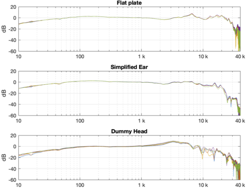
Figure 4. One measurement for each pair of headphones on each measurement system. The red curves are the dummy head and the blue curves are the artificial ear RELATIVE TO THE FLAT PLATE.
In Figure 4, I’m pretending that the flat plate is the “correct” system, and then I’m plotting the difference between the dummy head measurement (in red) and the artificial ear measurement (in blue) relative to it.
Again, it’s important to remember with these plots is that something that looks like a peak in the curve might actually be a dip in the “reference” curve. (The bump in the red lines around 2 – 3 kHz is an example of this…)
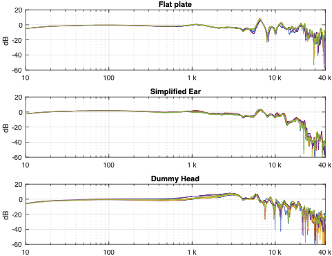
Of course, you could say “but you just said that we shouldn’t look at a single measurement”… which is correct. If we use the averages of all 5 measurements for each set and do the same plot, the result is Figure 5.
Figure 5. The average of all 5 measurements for each pair of headphones on each measurement system. The red curves are the dummy head and the blue curves are the artificial ear relative to the flat plate.
You can see there that, by using the averaged responses instead of individual measurements, the really sharp peaks and dips disappear, since they smooth each other out.
Comparing headphone types
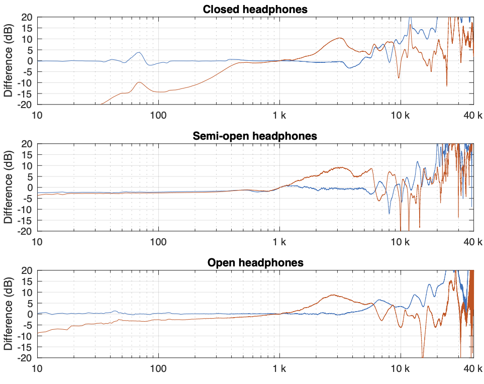
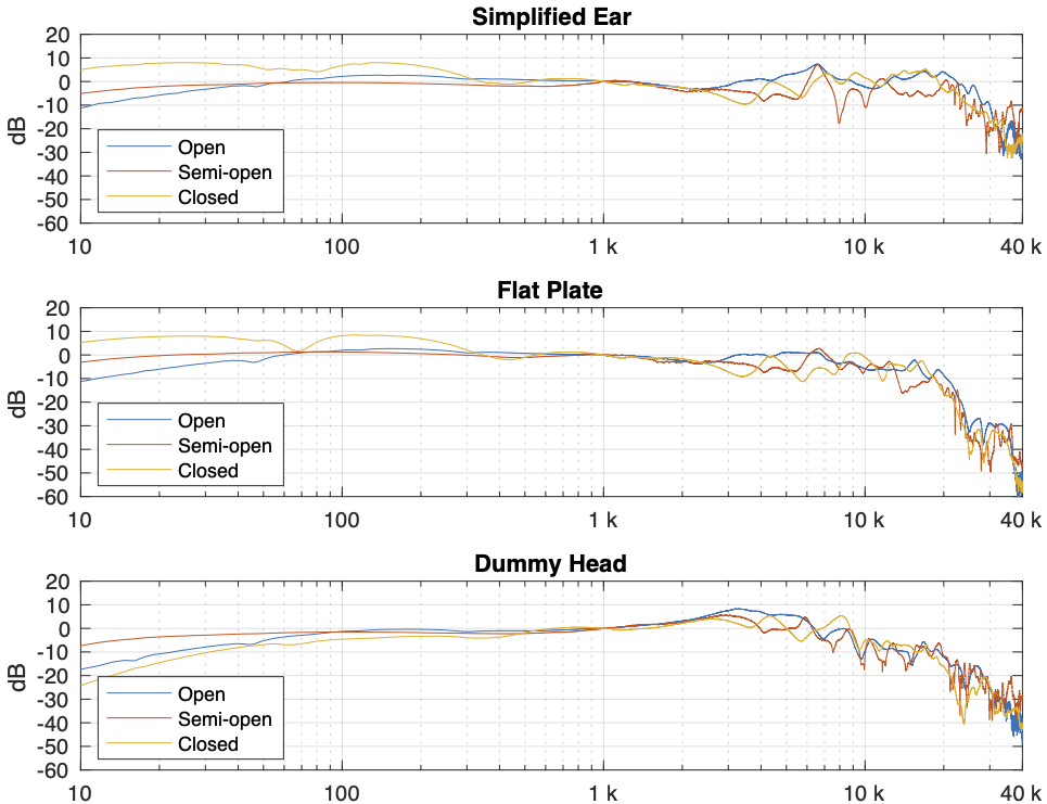
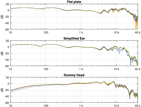
Things get even more complicated if you try to compare the headphones to each other using the measurement systems. Figure 6, below, shows the averages of the five measurements of each pair of headphones on each measurement system, plotted together on the same graphs (normalised to the levels at 1 kHz), one for each measurement system.
Figure 6: Comparing the three pairs of headphones on each measurement system.
This is actually a really important figure, since it shows that the same headphones measured the same way on different systems tell you very different things. For example, if you use the “simplified ear” or the “flat plate” system, you’ll believe that the closed headphones (the yellow line) is about 10 – 15 dB higher than the open headphones (the blue line) in the low frequency region. However, if you use the “dummy head” system, you’ll believe that the closed headphones (the yellow line) is about 5 – 10 dB lower than the open headphones (the blue line) in the low frequency region.
Which one is correct? They all are, even though they tell you different things. After all, it’s just data… The reason this happens is that one measurement system cannot be used to directly compare two different types of headphones because their acoustic impedances are different. With experience, you can learn to interpret the data you’re shown to get some idea of what’s going on. However, “experience” in that sentence means “years of correlating how the headphones sound with how the plots look with the measurement system(s) you use”. If you aren’t familiar with the measurement system and how it filters the measurement, then you won’t be able to interpret the data you get from it.
That said, you MIGHT be able to use one system to compare two different pairs of open headphones or two different pairs of closed headphones, but you can’t directly compare measurements of different headphone types (e.g. open and closed) reliably.
This also means that, if you subscribe to two different headphone magazines both of which use measurements as part of their reviews, and one of them uses a flat plate system while the other uses a dummy head, the same pairs of headphones might get opposite reviews in the two magazines…
Which review can you trust? Both of them – and neither of them.
Conclusions
Looking at these plots, you could come to the conclusion that you can’t trust anything, because no two measurements tell you the same things about the same devices. This is the incorrect conclusion to draw. These measurement systems are tools that we use to tell us something about the headphones on which we’re working. And people who use these tools daily know how to interpret the data they see from them. If something looks weird, they either expected it to look weird, or they run the measurement on another system to get a different view.
The danger comes when you make one measurement on one device and hold that up as The Truth. A result that you get from any one of these systems is not The Truth, but it is A Truth – you just need more information. If you’re only shown one measurement (or even an average of measurements) that was done on only one measurement system, then you should raise at least one eyebrow, and ask some questions about how that choice of system affects the plots that you see.
In many ways, it’s like looking at a recipe in a cookbook. You might be able to determine whether you might like or probably hate a dish by reading its description of ingredients and how to prepare it. But you cannot know how it’ll taste until you make it and put it in your mouth. And, if you cook like I do, it’ll be just a little different next time. It’s cooking – not a chemistry experiment. If you use headphones like I do, it’ll also be a little different next time because some days, I don’t wear my glasses, or I position the head band a little differently, so the leak around the ear cushion or the clamping force is a little different.
In Part 1, I talked about how any measurement of an audio device tells you something about how it behaves, but you need to know a LOT more than what you can learn from one measurements. This is especially true for a loudspeaker where you have the extra dimensions of physical space to consider.
Thought experiment: Fridges vs. Mosquitos
Consider a situation where you’re sitting at your kitchen table, and you can hear the compressor in your fridge humming/buzzing over on the other side of the room. If you make a small movement in your chair, the hum from the fridge sounds the same to you. This is partly because the distance from the fridge to you is much bigger than the changes in that distance that result from you shifting your butt.
Now think about the times you’ve been trying to sleep on a summer night, and there’s a mosquito that is flying near your ear. Very small changes in the location of that mosquito result in VERY big changes in how it sounds to you. This is because, relative to the distance to the mosquito, the changes in distance are big.
In other words, in the case of the fridge (that’s say, 3 m away) by moving 10 cm in your chair, you were changing the distance by about 3%, but the mosquito was changing its distance by more than 100% by moving just from 1 cm to 2 cm away.
In other words, a small change in distance makes a big change in sound when the distance is small to begin with.
The challenges of measuring headphones
The methods we use for measuring the magnitude response of a pair of headphones is similar to that used for measuring a loudspeaker. We send a measurement signal to the headphones from a computer, that signal comes out and is received by a microphone that sends its output back to the computer. The computer then is used to determine the difference between what it sent out and what came back. Simple, right?
Wrong.
The problems start with the fact that there are some fundamental differences between headphones and loudspeakers. For starters, there’s no “listening room” with headphones, so we don’t put a microphone 3 m away from the headphones: that wouldn’t make any sense. Instead, we put the headphones on some kind of a device that either simulates an ear, or a head, or a head with ears (with or without ear canals), and that device has a microphone (roughly) where your eardrum would be. Simple, right?
Wrong.
The problem in that sentence was the word “simulates”. How do you simulate an ear or a head or a head with ears? My ears are not shaped identically to yours or anyone else’s. My head is a different size than yours. I don’t have any hair, but you might. I wear glasses, but you might not. There are many things that make us different physically, so how can the device that we use to measure the headphones “simulate” us all? The simple answer to this question is “it can’t.”
This problem is compounded with the fact that measurement devices are usually made out of plastic and metal instead of human skin, so the headphones themselves “see” a different “acoustic load” on the measurement device than they do when they’re on a human head. (The people I work with call this your acoustic impedance.)
However, if your day job is to develop or test headphones, you need to use something to measure how they’re behaving. So, we do.
Headphone measurement systems
There are three basic types of devices that are used to measure headphones.
an artificial ear is typically a metal plate with a depression in the middle. At the bottom of the depression is a microphone. In theory, the acoustic impedance of this is similar to a human ear/pinna + the surrounding part of your head. In practice, this is impossible.
a headphone test fixture looks like a big metal can lying on its side (about the size of an old coffee can, for example) on a base. It might have flat metal sides, or it could have rubber pinnae (the fancy word for ears) mounted on it instead. In the centre of each circular end is a microphone.
a dummy head looks like a simplified model of a human head (typically a man’s head). It might have pinnae, but it might not. If it does, those pinnae might look very much like human ears, or they could look like simplified versions instead. There are microphones where you would expect them, and they might be at the bottom of ear canals, but you can also get dummy heads without ear canals where the microphones are flush with the side of the head.
The test system you use is up to you – but you have to know that they will all tell you something different. This is not only because each of them has a different acoustic response, but also because their different shapes and materials make the headphones themselves behave differently.
That last sentence is important to remember, not just for headphone measurement systems but also for you. If your head and my head are different from each other, AND your pinnae and my pinnae are different from each other, THEN, if I lend you my headphones, the headphones themselves will behave differently on your head than they do on my head. It’s not just our opinions of how they sound that are different – they actually sound different at our two sets of eardrums.
General headphone types
If I oversimplify headphone design, we can talk about two basic acoustical type of headphones: They can be closed (where the back of the diaphragm is enclosed in a sealed cabinet, and so the outside of the headphones is typically made of metal or plastic) or open (where the back of the diaphragm is exposed to the outside world, typically through a metal screen). I’d say that some kinds of headphones can be called semi-open, which just means that the screen has smaller (and/or fewer) holes in it, so there’s less acoustical “transparency” to the outside world.
Examples
To show that all these combinations are different, I took three pairs of headphones
open headphones
semi-open headphones
closed headphones
and I measured each of them on three test devices
artificial “simplified” ear
text fixture with a flat-plate
dummy head
In addition, to illustrate an additional issue (the “mosquito problem”), I did each of these 9 measurements 5 times, removing and replacing the headphones between each measurement. I was intentionally sloppy when placing the headphones on the devices, but kept my accuracy within ±5 mm of the “correct” location. I also changed the clamping force of the headphones on the test devices (by changing the extension of the headband to a random place each time) since this also has a measurable effect on the measured response.
Do not bother asking which headphones I measured or which test systems I used. I’m not telling, since it doesn’t matter. Not to me, anyway…
The raw results
I did these measurements using a 10-second sinusoidal sweep from 2 Hz to Nyquist, on a system running at 96 kHz. I’m plotting the magnitude responses with a range from 10 Hz to 40 kHz. However, since the sweep starts at 2 Hz, you can’t really trust the results below 20 Hz (a decade below the lowest frequency of interest is a good rule of thumb when using sine sweeps).
Figure 1: The “raw” magnitude responses of the open headphones measured 5 times each on the three systems
Figure 2: The “raw” magnitude responses of the semi-open headphones measured 5 times each on the three systems
Figure 3: The “raw” magnitude responses of the closed headphones measured 5 times each on the three systems
Looking at the results in the plots above, you can come to some very quick conclusions:
All of the measurements are different from each other, even when you’re looking at the same headphones on the same measurement device. This is especially true in the high frequency bands.
Each pair of headphones looks like it has a different response on each measurement system. For example, looking at Figure 3, the response of the headphones looks different when measured on a flat plate than on a dummy head.
The difference in the results of the systems are different with the different headphone types. For example, the three sets of plots for the “semi-open” headphones (Fig. 2) look more similar to each other than the three sets of plots for the “closed” headphones (Fig. 3)
the scale of these differences is big. Notice that we have an 80 dB scale on all plots… We’re not dealing with subtleties here…
In Part 3 of this series, we’ll dig into those raw results a little to compare and contrast them and talk a little about why they are as different as they are.
People who work in the audio industry use all kinds of different measurements to evaluate the performance of equipment. In many cases, the measurements we do are chosen because they’re easy to do (or because they were easy to do in “The Old Days”), and not because they accurately represent how the equipment actually behaves.
Magnitude response
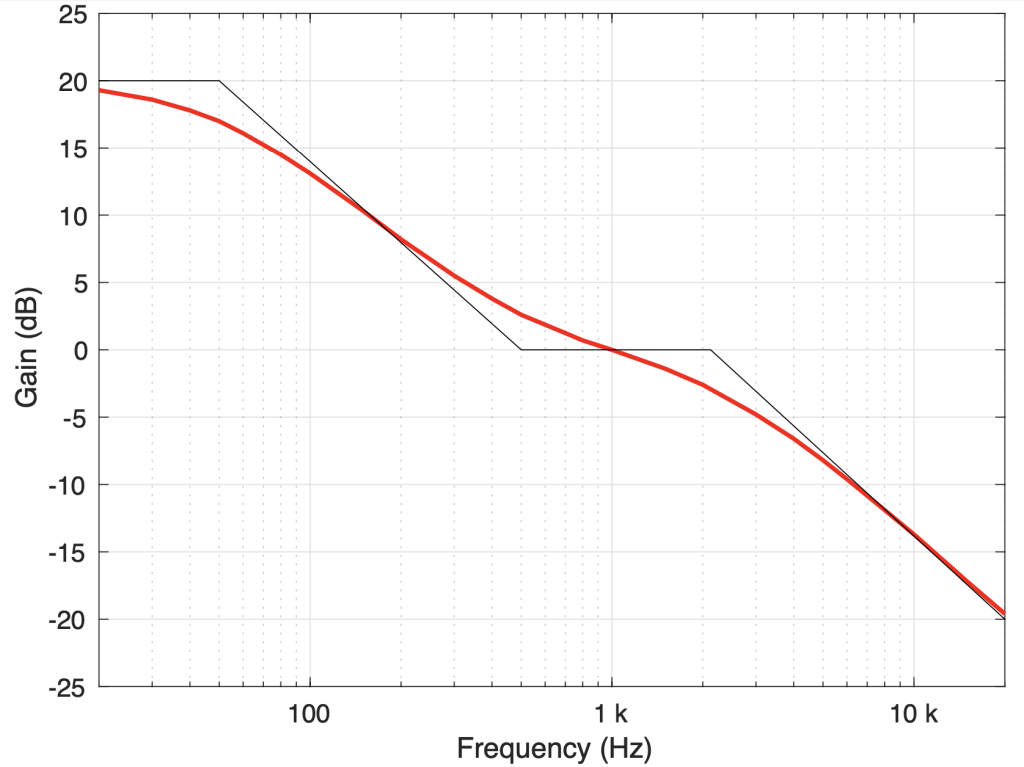
One simple example of this is what most people call a frequency response but what is actually a magnitude response. This is a measure of how the level of an audio signal is changed by the device under test (the “DUT”) as a function of frequency. For example, if you’re measuring a RIAA-spec preamplifier (used for converting a turntable’s pickup’s output to a “line” level signal), then it should have a magnitude response that looks like the red line in the plot in Figure 1.
Figure 1: The red line shows the correct magnitude response for the frequency-dependent filtering in a RIAA phono preamplifier.
This curve shows that, relative to a signal at 1 kHz, the lower the frequency, the more gain is applied to the signal and the higher the frequency, the more attenuation is applied to the signal. Note that this curve is normalised to the level at 1 kHz, which should actually be +40 dB higher if we were to include the frequency-independent gain of the system.
It’s important to remember that this plot shows us only one thing: the change in level caused by the DUT as a function of a change in frequency of the signal. What this plot does NOT show us is much, much more… For example:
We don’t know anything about the behaviour of the system outside the boundaries of this plot.
We don’t know anything about its phase response.
We don’t know anything about how loud the noise of the DUT is.
We don’t know if this plot is true if we were to measure the DUT at a different input level.
We don’t know whether the DUT would have a different behaviour if the device that was feeding it had a different output impedance.
We don’t know whether the DUT would have a different behaviour if the device that it was feeding had a different input impedance.
We don’t know anything about whether the signal has any non-linear distortion artefacts. (Notice that I didn’t say “…whether the signal is distorted” because we know it’s distorted, since the output of the DUT is not the same as the input of the DUT. Any change in the signal is a form of distortion of the signal.)
I’m not saying that a simple magnitude response plot of a DUT is not useful. I’m just saying that it’s not enough information. It’s like asking for the temperature of a cup of coffee. It’s useful information, but it doesn’t tell you enough to know whether you’re going to enjoy drinking it (unless, of course, you hate coffee…)
This problem gets even worse when you’re measuring the acoustic output of a device like a loudspeaker or a pair of headphones, for example. (The acoustic input of a microphone is a similar problem in the opposite direction.)
Let’s start by thinking about a loudspeaker’s output in real life.
You have a device that radiates sound in space in all directions. Let’s look at that space from the loudspeaker’s perspective and say that this means an angle of rotation around the loudspeaker, and an angle of elevation above/below the loudspeaker. That makes two dimensions.
If we’re talking about the loudspeaker’s magnitude response, then we’re looking at its output level (one dimension) as a function of frequency (one more dimension).
That speaker is (usually) in a room, and you’re probably also there too. We can then that this is in three-dimensional space when we talk about the walls, floor, ceiling, and your location inside that space.
Since the surfaces in the room reflect the audio signal, then the time at which the signal arrives at the listening position must also be considered. The “sound” of a loudspeaker at a listening position before the first reflection arrives is different than after a bunch of reflections are coming in and the room has started resonating as well. So, time adds one more dimension to the problem.
We’ll ignore the non-linear distortion artefacts produced by the loudspeaker and the fact that they radiate in different directions differently, since it’s already complicated enough… However, if we were to add things like changes in the response due to temperature of the voice coil or directionally-dependent distortion artefacts like breakup, this would wind up being a much longer discussion…
So, just looking at the small list of “usual suspects” above, we can see that evaluating the sound of a single loudspeaker in a listening room is at least an 8-dimensional problem. And this doesn’t even take things like 2-channel stereo or 7.1.4 multichannel or whether you’re listening to Aretha Franklin or Stockhausen into account…
In other words, it’s complicated. So, we use reductionism to try to start to get an idea of what’s going on. We put a microphone directly in front of a loudspeaker and measure its magnitude response at one level using one kind of test signal (e.g. a swept sine wave or an MLS) and we remove all the room’s reflections somehow. This reduces our 8-dimensional problem to a 2-dimensional version: we have level as a function of frequency and nothing else, since we’ve chosen to throw away everything else by the way we did the measurement.
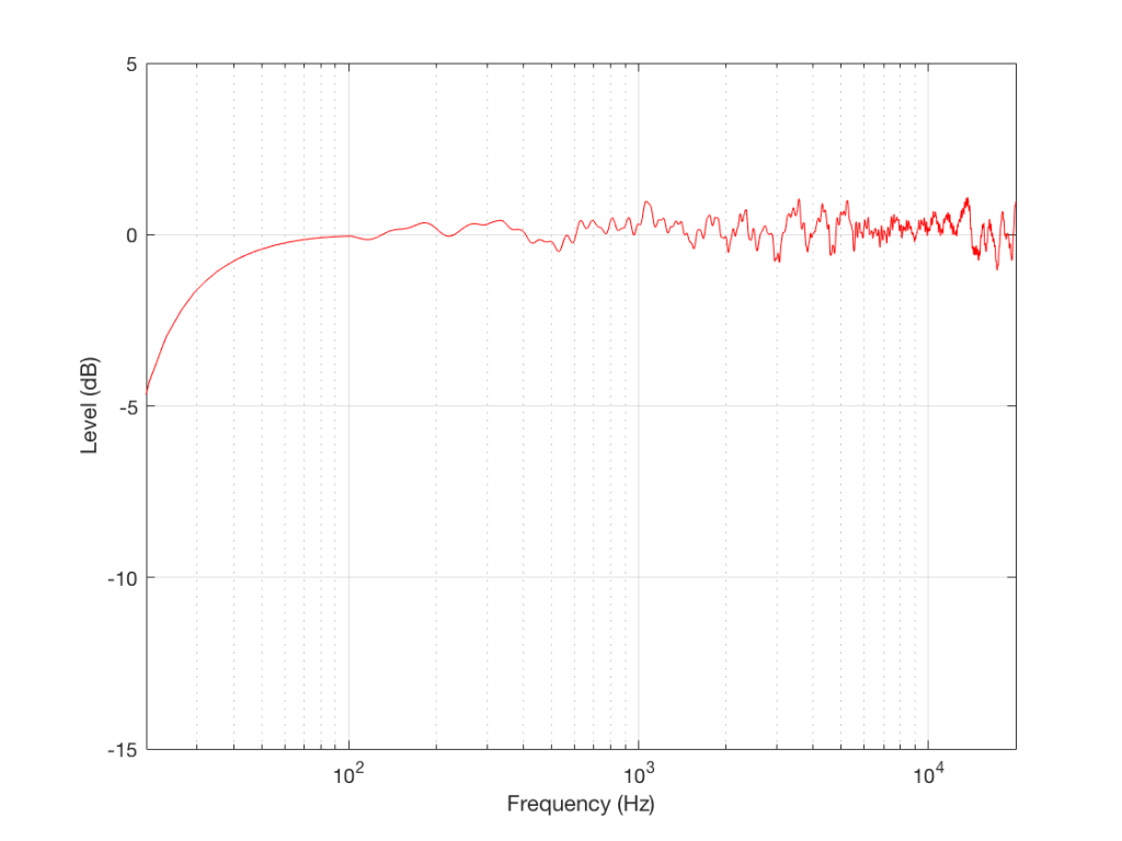
Figure 2: The on-axis, free-field magnitude response of a loudspeaker.
For example, take a look at the magnitude response shown in Figure 2, which is a real measurement of a real loudspeaker. This measurement was performed using a swept-sine (a sinusoidal wave with a frequency that changes smoothly over time, typically from low to high) with a microphone on-axis to the loudspeaker at a distance of 3 m. The measurement was time-windowed to remove the room reflections, and therefore can be considered to be a “free field” (a sound field that is free of reflections) measurement. However, the roll-off in the low end is actually a combination of the actual response of the loudspeaker and the artefacts of using a shorter time window. (We would have needed to use a much bigger room to get less influence from the time windowing.)
So, this plot ONLY tells us how the loudspeaker behaves at one point in infinite space, when we’re ONLY asking “how does the level of the loudspeaker’s output vary with changes in frequency and we ONLY play sinusoidal signals at one level.” This is all useful information, but we need to know more – otherwise, we’ll jump to conclusions about whether this loudspeaker sounds “good” or not.
Just like looking at ONLY the temperature of a cup of coffee, this doesn’t give us enough of the story to know how the loudspeaker will “sound” (no matter what a magazine reviewer will try and tell you…).
In other words, if we use reductionism to understand the problem, you simplify the question so much that the problem you wind up understanding is not the same as the thing you’re trying to understand in the first place.
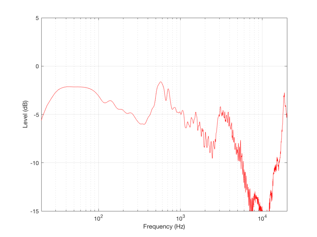
For example, if we measure that same loudspeaker at a different angle (by rotating the loudspeaker and leaving the microphone in place) we’ll see a magnitude response like the one shown in Figure 3.
Figure 3: The free-field magnitude response of the same loudspeaker, measured at 90º off-axis.
This magnitude response is the output of the same loudspeaker at 90º off-axis, which might be what’s heading towards your side-wall. If your side wall is perfectly reflective, then this is therefore the magnitude response of your first reflection, which might be a bad thing if you think that it’s important.
So, when you’re looking at any one measurement of anything, you don’t have enough information to know enough to make a general evaluation. However, unfortunately, many people will run with this information and make the evaluation anyway. It’s data, and data doesn’t lie, so this tells the truth, right?
Wrong. Because it’s only a portion of the total truth.
For example, you can say that “organic food is good for me” but I have an allergy to peanuts. So if I eat organic peanuts, I have about 20 minutes to get to a hospital. Much longer than that and I need a funeral home instead. “Organic” is true, but not enough information for me to know whether or not it’ll be an uneventful meal.
In Part 3, I showed that a magnitude responses calculated from impulse responses produced by the MLS and swept sine methods produce different results when the measurement signals themselves are distorted.
In this posting, I’ll focus on the swept sine method which showed that the apparent magnitude response of the system looked like a strange version of a low shelving filter, but there’s a really easy explanation for this that goes back to something I wrote in Part 1.
The way these systems work is to cross-correlate the signal that comes back from the DUT with the signal that was sent to it. Cross-correlation (in this case) is a bit of math that tells you how similar two signals are when they’re compared over a change in time (sort of…). So, if the incoming signal is identical to the outgoing signal at one moment in time but no other, then the result (the impulse response) looks like a spike that hits 1 (meaning “identical”) at one moment, and is 0 (meaning “not at all alike in any way…”) at all other times.
However, one important thing to remember is that both an MLS signal and a swept sine wave take some time to play. So, on the one hand, it’s a little weird to think of a 10-second sweep or MLS signal being converted to a theoretically-infinitely short impulse. On the other hand, this can be done if the system doesn’t change in time and therefore never changes: something we call a Linear Time-Invariant (or LTI) system.
But what happens if the DUT’s behaviour DOES change over time? Then things get weird.
At the end of Part 1, I said
For both the MLS and the sine sweep, I’m applying a pre-emphasis filter to the signal sent to the DUT and a reciprocal de-emphasis filter to the signal coming from it. This puts a bass-heavy tilt on the signal to be more like the spectrum of music. However, it’s not a “pinking” filter, which would cause a loss of SNR due to the frequency-domain slope starting at too low a frequency.
Then, in Part 2 I said that, to distort the signals, I
look for the peak value of the measurement signal coming into the DUT, and then clip it.
It’s the combination of these two things that results in the magnitude response of the system measured using a swept sine wave looking the way it does.
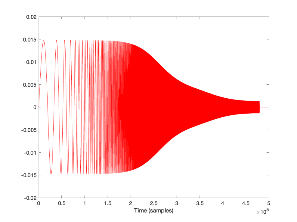
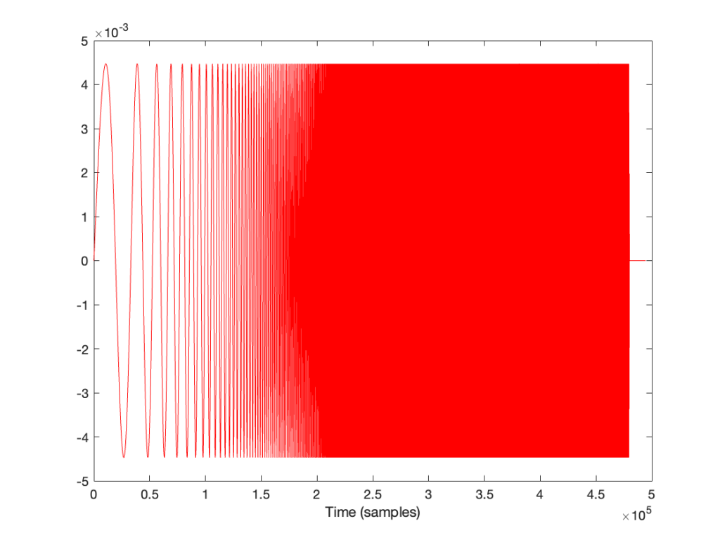
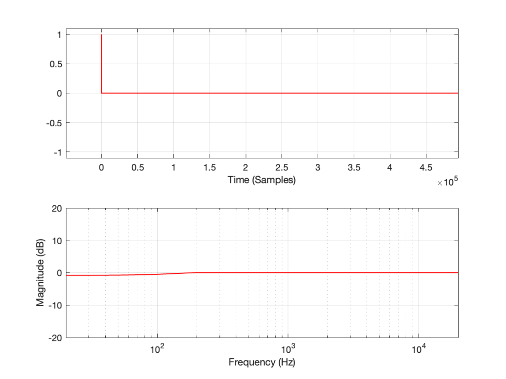
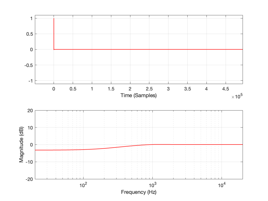
If I look at the signal that I actually send to the input of the DUT, it looks like this:
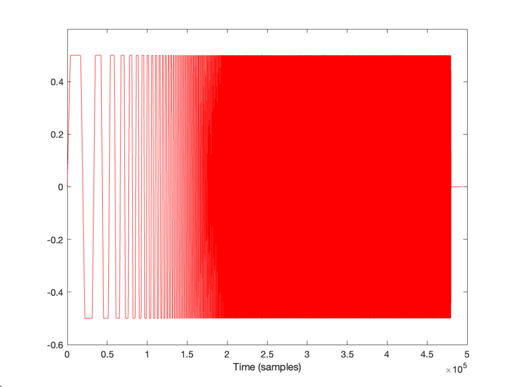
I’m normalising this to have a maximum value of 1 and then clipping it at some value like ±0.5, for example, like this:
So, it should be immediately obvious that, by choosing to clip the signal at 1/2 of the maximum value of the whole sweep, I’m not clipping the entire thing. I’m only distorting signals below some frequency that is related to the level at which I’m clipping. The harder I clip, the higher the frequency I mess up.
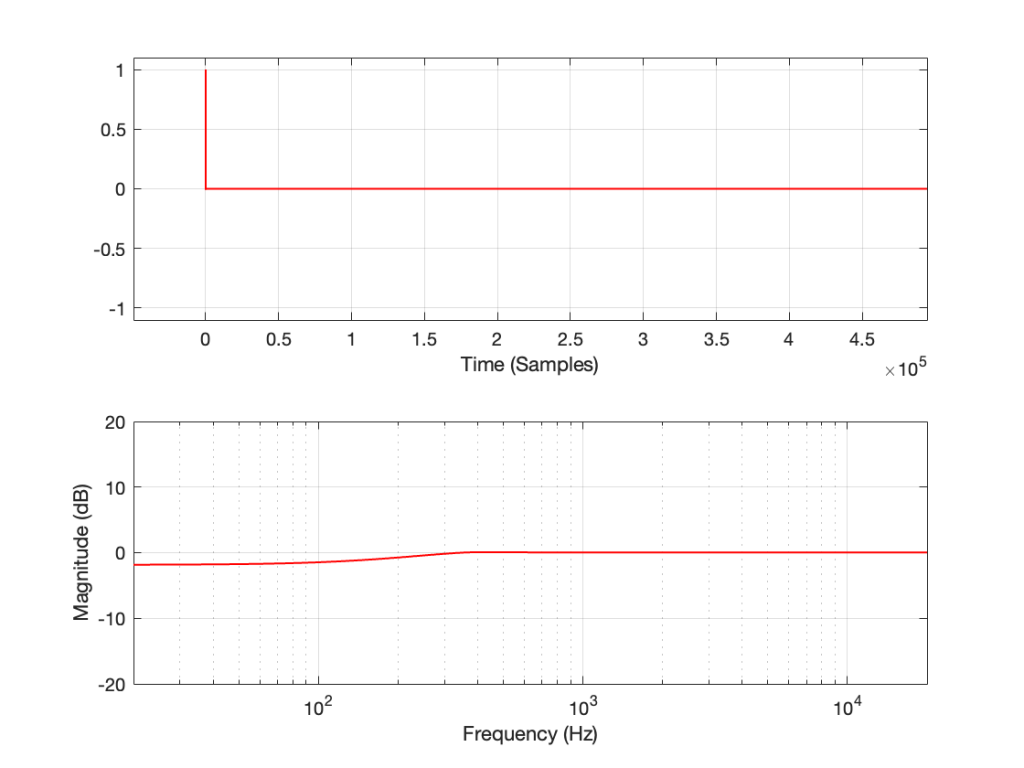
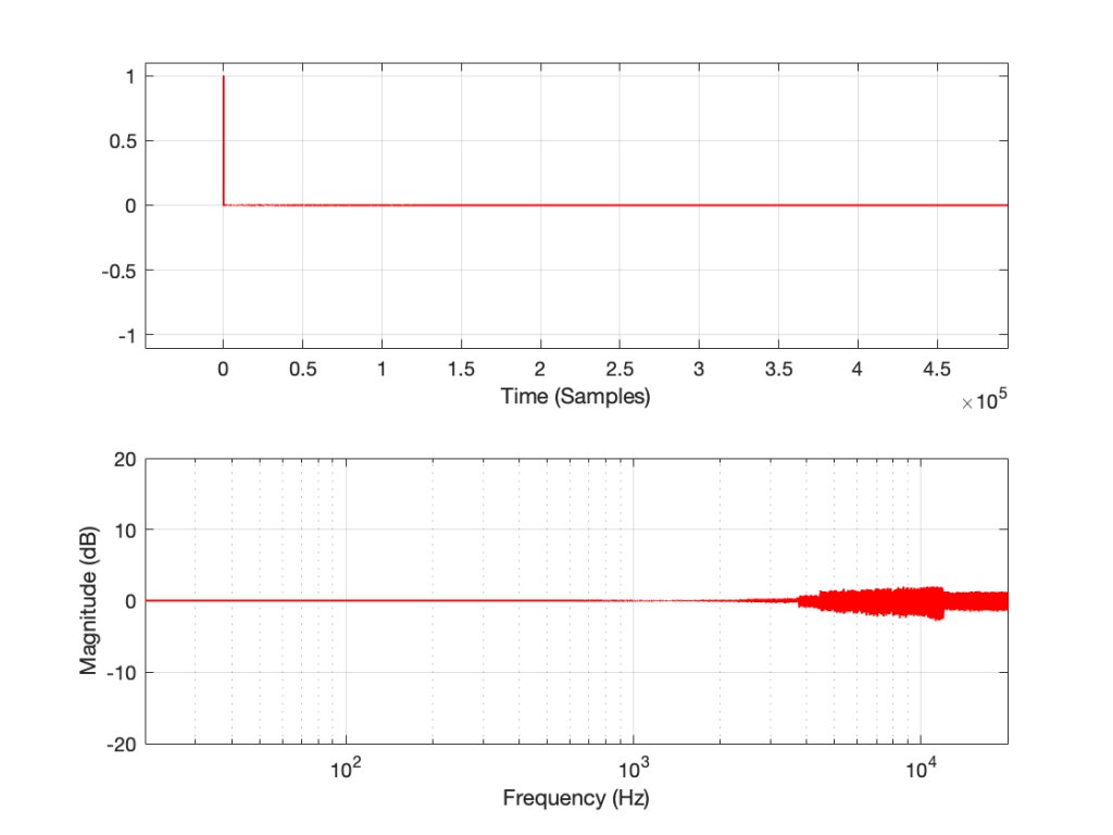
This is why, when we look at the magnitude response, it looks like this:
In the very low frequencies, the magnitude response is flat, but lower than expected, because the signal is clipped by the same amount. In the high frequencies, the signal is not clipped at all, so everything is behaving. In between these two bands, there is a transition between “not-behaving” and “behaving”.
This means that
if the signal I was sending into the system was clipped by the same amount at all frequencies, OR
if the pre-emphasis wasn’t applied to the signal, boosting the low frequencies
Then the magnitude response would look almost flat, but lower than expected (by the amount that is related to how much it’s clipped). In other words, we would (mostly) see the linear response of the system, even though it was behaving non-linearly – almost like if we had only sent a click through it.
However, if we chose to not apply the pre-emphasis to the signal, then the DUT wouldn’t be behaving the way it normally does, since this is very roughly equivalent to the spectral balance of music. For example, if you send a swept sine wave from 20 Hz to 20,000 Hz to a loudspeaker without applying that bass boost, you’ll could either get almost nothing out of your woofer, or you’ll burn out your tweeter (depending on how loudly you’re playing the sweep).
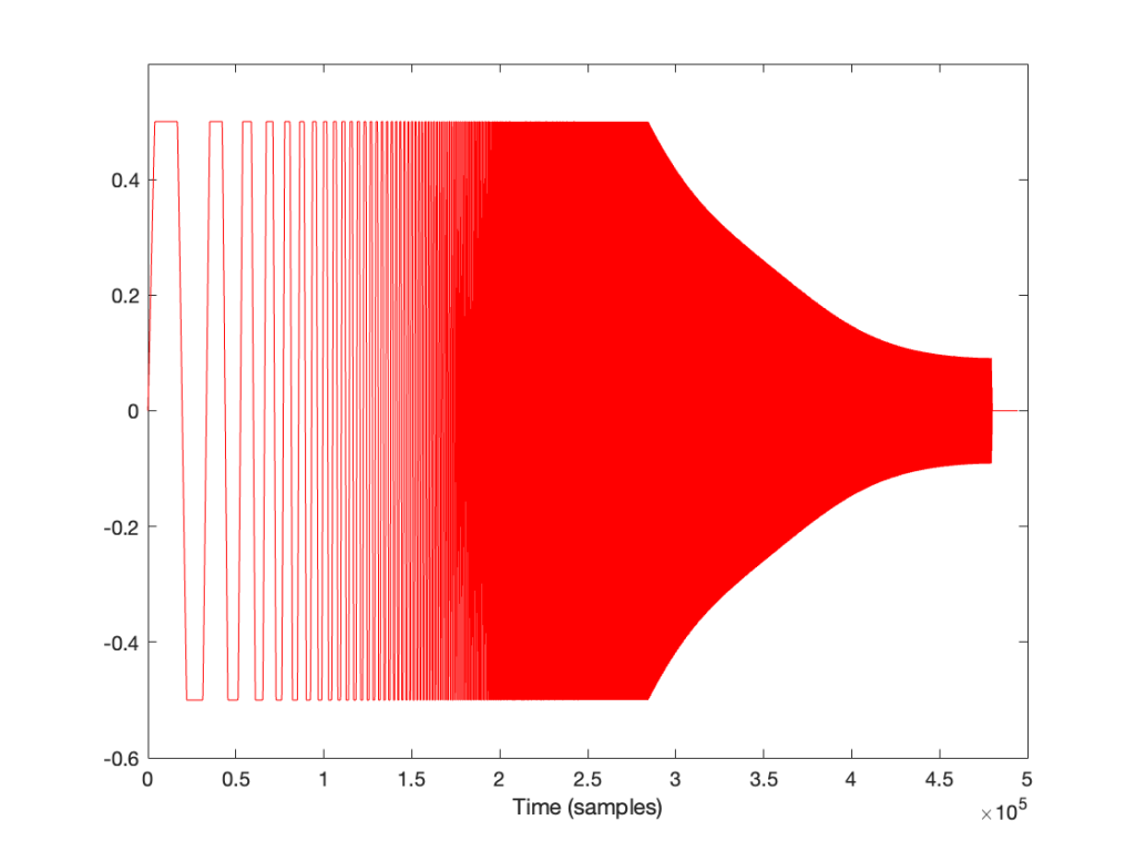
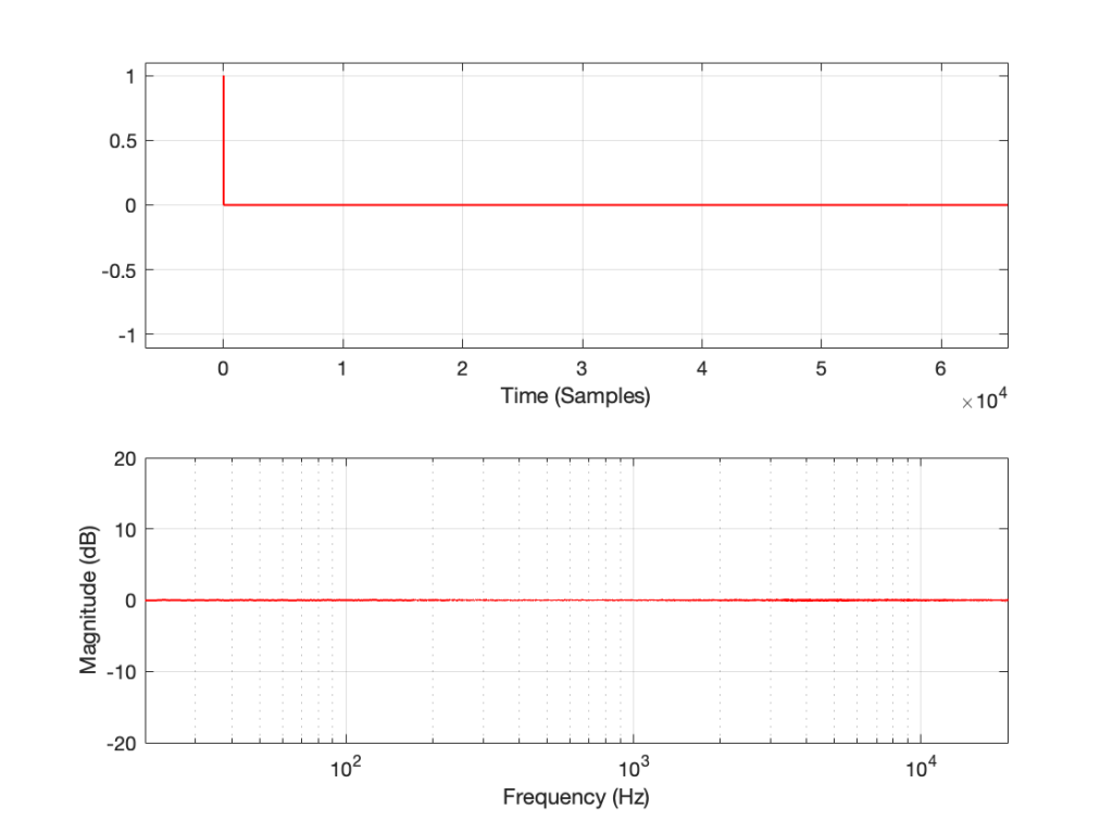
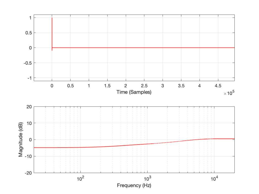
How does the result look without the pre-emphasis filter applied to the swept sine wave? For example, if we sent this to the DUT:
… and then we clipped it at 1/2 the maximum value, so it looks like this:
(notice that everything is clipped)
then the impulse response and magnitude response look like this instead:
… which is more similar to the results when we clip the MLS measurement signal in that we see the effects on the top end of the signal. However, it’s still not a real representation of how the DUT “sounds” whatever that means…
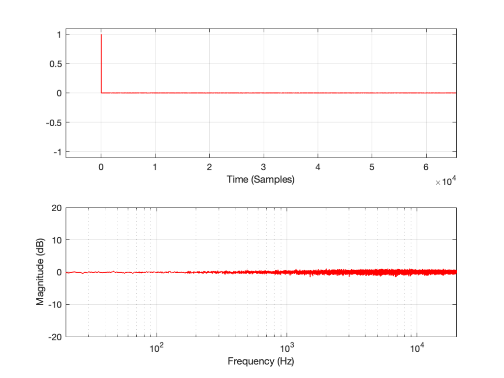
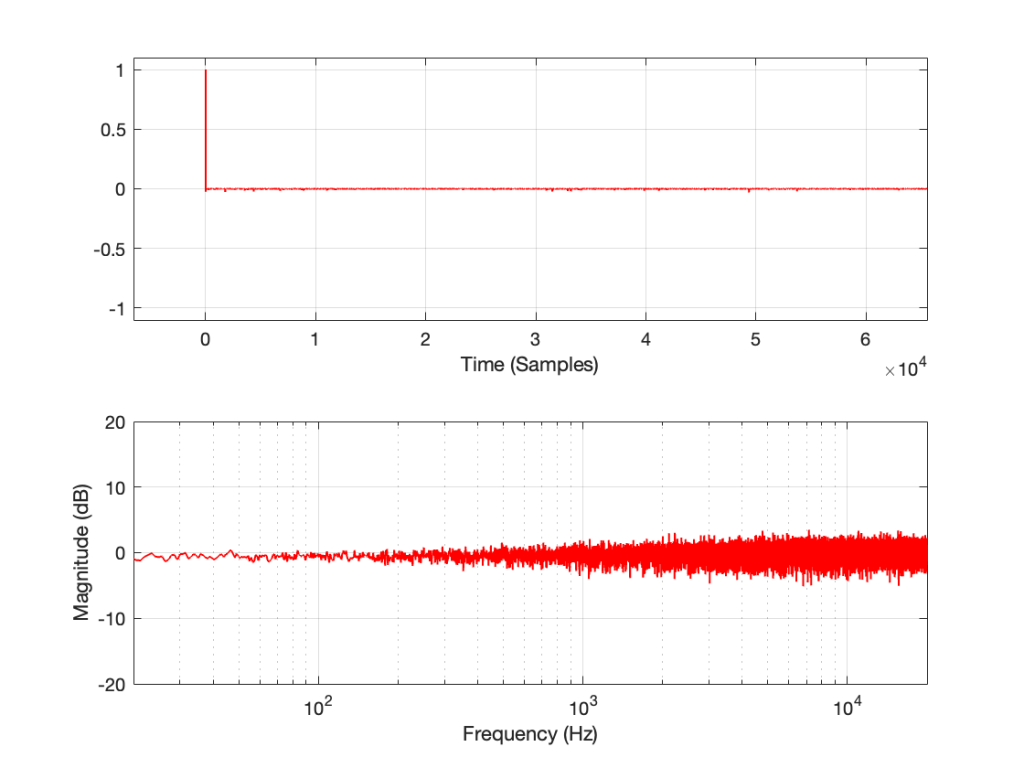
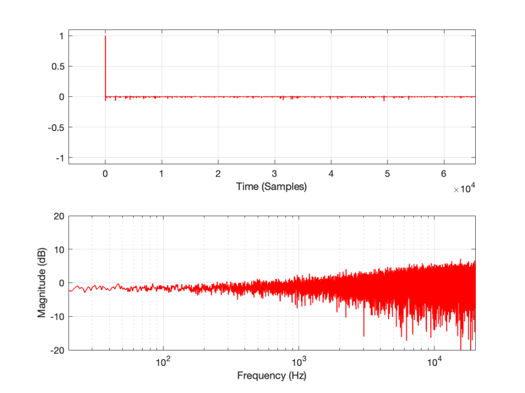
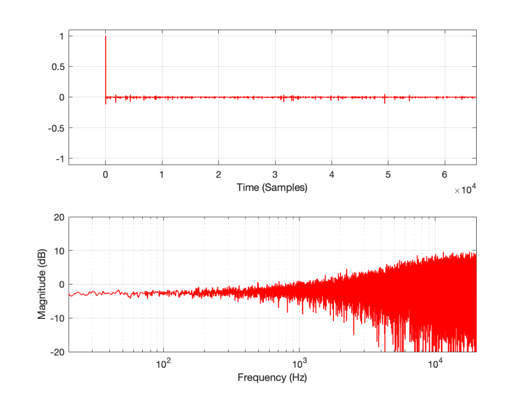
This posting will just be some more examples of the artefacts caused by symmetrical clipping of the measurement signal for the MLS and swept-sine methods, clipping at different levels.
Remember that the clip level is relative to the peak level of the measurement signal.
MLS
MLS, clipping at 0.9 of peak level
MLS, clipping at 0.7 of peak level
MLS, clipping at 0.5 of peak level
MLS, clipping at 0.3 of peak level
MLS, clipping at 0.1 of peak level
Swept Sine
Swept Sine, clipping at 0.9 of peak level
Swept Sine, clipping at 0.7 of peak level
Swept Sine, clipping at 0.5 of peak level
Swept Sine, clipping at 0.3 of peak level
Swept Sine, clipping at 0.1 of peak level
The take-home message here is that, although both the MLS and the swept sine methods suffer from showing you strange things when the DUT is clipping, the swept sine method is much less cranky…
In the next posting, I’ll explain why this is the case.
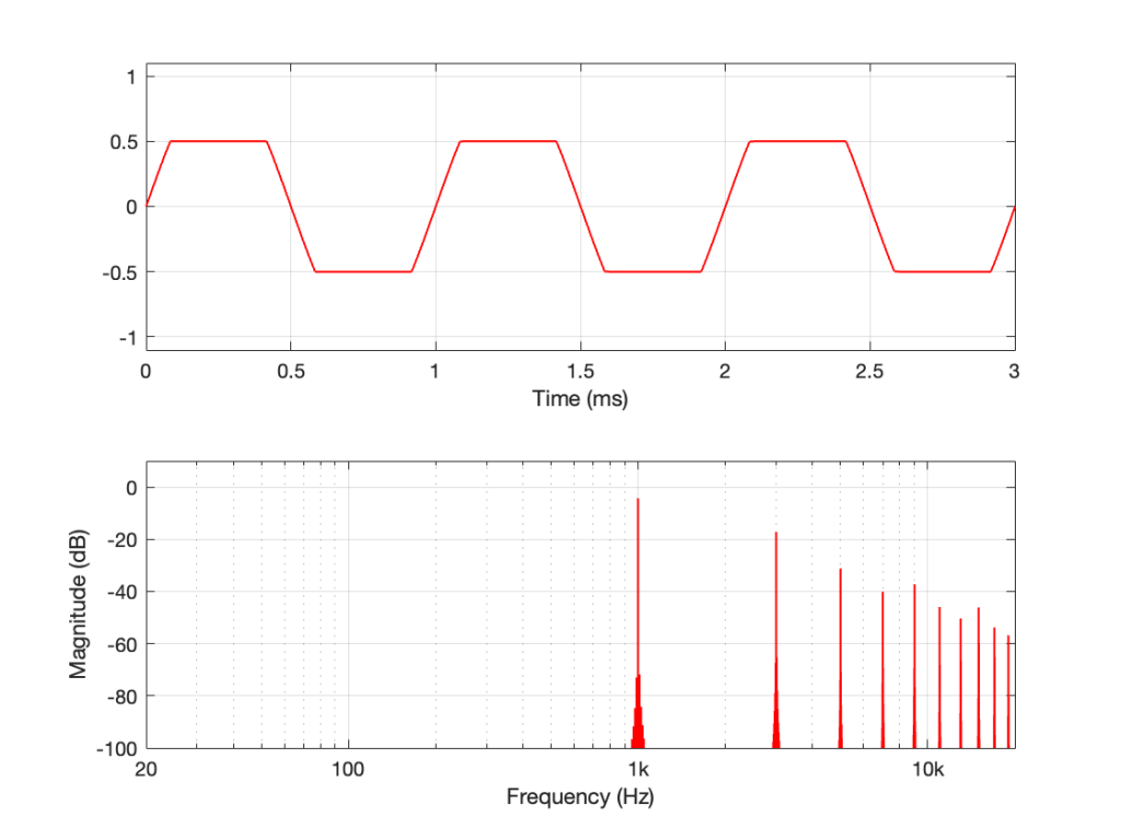
Let’s make a DUT with a simple distortion problem: It clips the signal symmetrically at 0.5 of the peak value of the signal, so if I send in a sine wave at 1 kHz, it looks like this:
Figure 1: An example of a symmetrically-clipped sine wave with a fundamental frequency of 1 kHz.
Now, to be fair, what I’m REALLY doing here is to look for the peak value of the measurement signal coming into the DUT, and then clipping it. This would be equivalent to doing a measurement of the DUT and adjusting the input gain so that it looks like a peak level of – 6 dB relative to maximum is coming in.
Also, because what I’m about to do through this series is going to have radical effects on the level after processing, I’m normalising the levels. So, some things won’t look right from a perspective of how-loud-it-appears-to-be.
If I measure that DUT using the three methods, the results look like this:
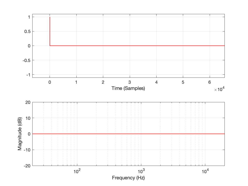
Figure 2: The impulse response of a clipping DUT, measured with an impulse (plot has been normalised for level).
Figure 3: The impulse response of a clipping DUT, measured with an MLS sequence (plot has been normalised for level).
Figure 4: The impulse response of a clipping DUT, measured with a swept sine (plot has been normalised for level).
As can easily be seen above, the three systems show very different responses. So, unlike what I claimed this post (which is admittedly over-simplified, although intentionally so to make a point…), the fact that they are measuring the impulse response does not mean that we can’t see the effects of the non-linear response. We can obviously see artefacts in the linear response that are caused by the distortion, but those artefacts don’t look like distortion, and they don’t really show us the real linear response.