
Pop music is bad and it’s your fault

An interesting little video on the obvious…
This article describes and criticises the publication from the Spanish National Research Council that’s mentioned in the video.
B&O Tech: The History of BeoLit
Ronny Kaas og Hans Vestergaard Nielsen: Specialists on the history of Bang & Olufsen, talking about the BeoLit series (in Danish).

B&O Tech: How B&O Makes a Loudspeaker – Part 2/2
#31 in a series of articles about the technology behind Bang & Olufsen loudspeakers
from www.recordere.dk when they visited Struer for the BeoLab 20 launch.
B&O Tech: How B&O Makes a loudspeaker: Part 1/2
#30 in a series of articles about the technology behind Bang & Olufsen loudspeakers
from www.recordere.dk when they visited Struer for the BeoLab 20 launch.
B&O Tech: Reading Spec’s – Part 1
#28 in a series of articles about the technology behind Bang & Olufsen loudspeakers
Introduction
Occasionally, I read other people’s blogs and forum postings to see what’s happening outside my little world. This week, I came across this page in which one of the contributors made some comments about B&O’s loudspeaker specifications – or, more precisely, the lack of them – or the lack of precision in them – particularly with respect to the Frequency Range specifications.
So, this posting will be an attempt to explain how we determine the frequency range of our loudspeakers.
Bandwidth (also known as “Frequency Range”)
Ask any first-year electrical engineering student to explain how to find the “bandwidth” of an audio product and they’ll probably all tell you the same thing – which will be something like the following:
- Measure the magnitude response (what many people call the “frequency response”) of the product.
- Find the peak in the magnitude response
- Going upwards in frequency, find the point where the magnitude drops by 3.01 dB relative to the peak.
- Going downwards in frequency, find the point where the magnitude drops by 3.01 dB relative to the peak.
- Subtract the lower frequency from the upper frequency and you get the bandwidth.
(If you’re curious, the 3.01 dB threshold is chosen because -3.01 dB is equivalent to one-half of the power of the peak. This is why the -3.01 dB points are also known as a the “half-power points”)
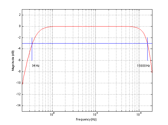
Figure 1 shows a pretty typical looking curve for an audio device (admittedly, not a very good one…). The magnitude response is flat enough, and it extends down to 34 Hz and up to 15.6 kHz.
This same technique can be used to find the bandwidth of an audio processing device, as is shown in Figure 2.

Loudspeaker Frequency Range
Let’s try applying that same method used for audio “black boxes” on a loudspeaker. We’ll measure the on-axis magnitude response of the loudspeaker in a free field (one without reflections), and find the frequencies where the magnitude drops 3.01 dB below the peak value. An example of this is shown below.

Hmmmm… that didn’t turn out as nicely as I had hoped. It seems that (using this definition) the loudspeaker whose response is shown in Figure 3 has a Frequency Range of 7.3 kHz to 13.9 kHz. This is unfortunate, since it is not a tweeter – it’s a rather large, commerically-available, floor-standing loudspeaker with a rather good reputation.
Okay, maybe we’re being too stringent. Let’s say that, instead of defining the Frequency Range as the area between the – 3 / + 0 dB points, we’ll make it ± 3 dB instead. Figure 4 shows the same loudspeaker with that version of Frequency Range.

Great- it got better! Now the Frequency Range of this loudspeaker (under the new ±3 dB definition) is from 2.2 kHz to 15.9 kHz. On paper, that still makes it a tweeter – so we’re still in trouble here. Note that I have scaled the magnitude response here to “help” the loudspeaker as much as I can by putting the peak in the magnitude response on the + 3 dB line. If I had not done this (for example, if I had said “±3 dB relative to the magnitude at 1 kHz” the numbers would certainly not get better…)
Let’s try the same definition on a different loudspeaker – shown in Figure 5.

This loudspeaker (also a commerically-available floor-standing model with a good reputation) has a Frequency Range (using the ± 3 dB points) of 5.4 kHz to 18.0 kHz. This ±3 dB definition isn’t working out very well. Let’s try one more loudspeaker to see what happens.

Yay! It worked! For loudspeaker #3, shown in Figure 5, the Frequency Range is from 83 Hz to 20.9 kHz. Ummmm… except that, of the 3 loudspeakers I measured for this experiment, this is, by far the smallest. It’s a little 2-way loudspeaker that I can easily lift with one hand whilst sipping a cup of coffee from the other (and I don’t work out – ever!)
So, what we have learned so far is that it’s better to buy a small loudspeaker than a big one, since it has a much wider frequency range. No, wait. that can’t be right…
Hmmmm… what if we were to smooth the magnitude responses? Maybe that would help…

That’s a little better, but Loudspeaker #1 (the black curve), still bottoms out in the midrange, causing its frequency range to resemble that of a tweeter. And Loudspeaker #2 loses out on the high end due to the peaks. (Note that, in this plot, I’ve scaled them all to have the same magnitude at 1 kHz – just trying something out to see if that helps. It didn’t.) How about more smoothing?

Got it! Now all of the loudspeakers’ responses have been smeared out enough… uh… adequately smoothed… to make our definition of Frequency Range have a little meaning. The “big” loudspeakers have wider Frequency Ranges than the “little” loudspeaker. So, we’ll just octave-smooth all of our measurements. Well… at least until we find another loudspeaker that needs even more smoothing…
Sidebar: In case you’re wondering: the three loudspeakers I’m talking about above are all commercially available products. One of the three is a Bang & Olufsen loudspeaker. Don’t bother asking which is which (or which B&O loudspeaker it is) – I’m not telling – mostly because it doesn’t matter.
The moral thus far…
Of course, the point that I’m trying to make here is that Frequency Range, like any specification for any audio device, needs to make sense. If we arbitrarily set some test method (i.e. “measure the on-axis magnitude response – and then smooth it”) and apply arbitrary criteria (i.e. ± 3 dB) then we may not get a useful description of the device’s behaviour.
So, at this point, you’re probably asking “Well… how does B&O measure Frequency Range?” Well, I’m glad you asked!
After we’re done with the sound design of the loudspeaker, we have to make sure it has the correct sensitivity. This is a measure of how loud it is for a given voltage at its input. So, we put the loudspeaker in the Cube and measure its final on-axis magnitude response.
I’ll illustrate this using a magnitude response that I invented, shown in Fig 8. Note that this response is not a real loudspeaker – it’s one that I invented just for the purposes of this discussion.

We then look at the average level of the magnitude response between 200 Hz and 2 kHz and adjust the gain in the signal processing of the loudspeaker to make the sensitivity what we want it to be. For almost all B&O loudspeakers, that sensitivity corresponds to an output level of 88 dB SPL for an input with a level of 125 mV RMS. (The only exceptions are BeoLab 1, BeoLab 5, and BeoLab 9 which produce 91 dB SPL for a 125 mV RMS input.)
So, after the gain has been adjusted, the magnitude response looks like Figure 9, below.

We then look for the frequencies that have a magnitude that are 10 dB lower than the average level between 200 Hz and 2 kHz. This is illustrated in Figure 10.

The values that correspond to the -10 dB points (relative to the average level between 200 Hz and 2 kHz) are the frequencies stated in the Frequency Range specification.
This is how B&O specifies Frequency Range for all of its loudspeakers. That way, you (and we) can directly compare their specifications to each other. Of course, some other manufacturer may (or probably will) use a different method – so you cannot use B&O’s Frequency Range specifications to compare to another company’s products. We don’t use a ±3 dB threshold, not only because this would require arbitrary smoothing in order to prevent weird things from happening (as I showed above) but also because the on-axis magnitude response of B&O loudspeakers is a result of the loudspeakers’ sound design (which includes a consideration of its power response) which means that, if you just look at the on-axis response, it might not be as flat as a magazine would lead you to believe it should be.
The Fine Print
1. The method I described above is a slightly simplified explanation of what we actually do – but the difference between what I said and the truth is irrelevant. The details are in the method we use to do the averaging – so it’s not really a big deal unless you’re actually writing the software that has to do the work.
2. We do this measurement of the Frequency Range using a signal with a level of 125 mV at the input of the loudspeaker. So, if your music is playing with a similar level (or lower) then you will have a loudspeaker that is performing as specified. However, if you play the music louder, the frequency range will change. In most cases, the low frequency limit will increase due to the ABL and thermal protection algorithms. The details of (1) how much it will increase, (2) what level of music will cause it to increase, and (3) what frequency content in the music will cause it to increase, are different from loudspeaker model to loudspeaker model. This was the root of some confusion for some people when they compare the frequency range of the BeoLab 12-3 to the BeoLab 12-2. These two loudspeakers have almost identical low frequency cutoffs, despite the fact that one of them has 2 woofers and the other has only 1. At “normal” listening levels, they have both been tuned to have similar magnitude responses – however, as you turn up the volume, the BeoLab 12-2 will lose bass earlier than the BeoLab 12-3.
3. Subwoofers are different – since it doesn’t make sense to try and find the average magnitude response of a subwoofer between 200 Hz and 2 kHz.
Quality over Quantity?
Plenty to worry about…
NASA’s World Observatory World of Change
UK legalises personal media servers…
B&O Tech: Near… Far…
#27 in a series of articles about the technology behind Bang & Olufsen loudspeakers
Introduction
To begin with, please watch the following video.
One thing to notice is how they made Grover sound near and far. Two things change in his voice (yes, yes, I know. It’s not ACTUALLY Grover’s voice. It’s really Yoda’s). The first change is the level – but if you’re focus on only that you’ll notice that it doesn’t really change so much. Grover is a little louder when he’s near than when he’s far. However, there’s another change that’s more important – the level of the reverberation relative to the level of the “dry” voice (what recording engineers sometimes call the “wet/dry mix”). When Grover is near, the sound is quite “dry” – there’s very little reverberation. When Grover is far, you hear much more of the room (more likely actually a spring or a plate reverb unit, given that this was made in the 1970’s).
This is a trick that has been used by recording engineers for decades. You can simulate distance in a mix by adding reverb to the sound. For example, listen to the drums and horns in the studio version of Penguins by Lyle Lovett. Then listen to the live version of the same people playing the same tune. Of course, there are lots of things (other than reverb) that are different between these two recordings – but it’s a good start for a comparison. As another example, compare this recording to this recording. Of course, these are different recordings of different people singing different songs – but the thing to listen for is the wet/dry mix and the perception of distance in the mix. Another example is this recording compared to this recording.
So, why does this trick work? The answer lies inside your brain – so we’ll have to look there first.
Distance Perception in the Mix
If you’re in a room with your eyes closed, and someone in the room starts talking to you, you’ll be pretty good at estimating where they are in the room – both in terms of angular location (you can point at them) and distance. This is true, even if you’ve never been in the room before. Very generally speaking, what’s going on here is that your brain is automatically comparing:
- the two sounds coming into your two ears – the difference between these two signals tells you a lot about which direction the sound is coming from, AND
- the direct sound from the source to the reflected sound coming from the room. This comparison gives you lots of information about a sound source’s distance and the size and acoustical characteristics of the room itself.
If we do the same thing in an anechoic chamber (a room where there are no echoes, because the walls absorb all sound) you will still be good at estimating the angle to the sound source (because you still have two ears), but you will fail miserably at the distance estimation (because there are no reflections to help you figure this out).
If you want to try this in real life, go outside (away from any big walls), close your eyes, and try to focus on how far away the sound sources appear to be. You have to work a little to force yourself to ignore the fact that you know where they really are – but when you do, you’ll find that things sound much closer than they are. This is because outdoors is relatively anechoic. If you go to the middle of a frozen lake that’s covered in fluffy snow, you’ll come as close as you’ll probably get to an anechoic environment in real life. (unless you do this as a hobby)

So, the moral of the story here is that, if you’re doing a recording and you want to make things sound far away, add reflections and reverberation – or at least make them louder and the direct sound quieter.
Distance Perception in the Listening Room
Let’s go back to that example of the studio recording of Lyle Lovett recording of Penguins. If you sit in your listening room and play that recording out of a pair of loudspeakers, how far away do the drums and horns sound relative to you? Now we’re not talking about whether one sounds further away than the other within the mix. I’m asking, “If you close your eyes and try to guess how far away the snare drum is from your listening position – what would you guess?”
For many people, the answer will be approximately as far away as the loudspeakers. So, if your loudspeakers are 3 m from the listening position, the horns (in that recording) will sound about 3 m away as well. However, this is not necessarily the case. Remember that the perception of distance is dependent on the relative levels of the direct and reflected sounds at your ears. So, if you listen to that recording in an anechoic chamber, the horns will sound closer than the loudspeakers (because there are no reflections to tell you how far away things are). The more reflective the room’s surfaces, the more the horns will sound further away (but probably no further than the loudspeakers, since the recording is quite dry).
This effect can also be the result of the width of the loudspeaker’s directivity. For example, a loudspeaker that emits a very narrow beam (like a laser, assuming that were possible) would not send any sound towards the walls – only towards the listening position. So, this would have the same effect as having no reflection (because there is no sound going towards the sidewalls to reflect). In other words, the wider the dispersion of the sound from the loudspeaker (in a reflective room) the greater the apparent distance to the sound (but no greater than the distance to the loudspeakers, assuming that the recording is “dry”).
Loudspeaker directivity
So, we’ve established that the apparent distance to a phantom image in a recording is, in part, and in some (perhaps most) cases, dependent on the loudspeaker’s directivity. So, let’s concentrate on that for a bit.
Let’s build a very simple loudspeaker. It’s a model that has been used to simulate the behaviour of a real loudspeaker, so I don’t feel too bad about over-simplifying too much here. We’ll build an infinite wall with a piston in it that moves in and out. For example:
Here, you can see the piston (in red) moving in and out of the wall (in grey) with the resulting sound waves (the expanding curves) moving outwards in the air (in white).
The problem with this video is that it’s a little too simple. We also have to consider how the sound radiation off the front of the piston will be different at different frequencies. Without getting into the physics of “why” (if you’re interested in that, you can look here or here or here for an explanation) a piston has a general behaviour with repeat to the radiation patten of the sound wave it generates. Generally, the higher the frequency, the narrower the “beam” of sound. At low frequencies, there is basically no beam – the sound is emitted in all directions equally. At high frequencies, the beam to be very narrow.
The question then is “how high a frequency is ‘high’?” The answer to that lies in the diameter of the piston (or the diameter of the loudspeaker driver, if we’re interested in real life). For example, take a look at Figure 1, below.

Figure 1 shows how loud a signal will be if you measure it at different directions relative to the face of a piston that is 10″ (25.4 cm) in diameter. Two frequencies are shown – 100 Hz (the blue curve) and 1.5 kHz (the green curve). Both curves have been normalised to be the same level (100 dB SPL – although the actual value really doesn’t matter) on axis (at 0°). As you can see in the plot, as you move off to the side (either to 90° or 270°) the blue curve stays at 100 dB SPL. So, no matter what your angle relative to on-axis to the woofer, 100 Hz will be the same level (assuming that you maintain your distance). However, look at the green curve in comparison. As you move off to the side, the 1.5 kHz tone drops by more than 20 dB. Remember that this also means that (if the loudspeaker is pointing at you and the sidewall is to the side of the loudspeaker) then 100 Hz and 1.5 kHz will both get to you at the same level. However, the reflection off the wall will have 20 dB more level at 100 Hz than at 1.5 kHz. This also means, generally, that there is more energy in the room at 100 Hz than there is at 1.5 kHz because, if you consider the entire radiation of the loudspeaker averaged over all directions at the same time the lower frequency is louder in more places.
This, in turn, means that, if all you have is a 10″ woofer and you play music, you’ll notice that the high frequency content sounds closer to you in the room than the low frequency content.
If the loudspeaker driver is smaller, the effect is the same, the only difference is that the effect happens at a higher frequency. For example, Figure 2, below shows the off-axis response for two frequencies emitted by a 1″ (2.54 cm) diameter piston (i.e. a tweeter).

Notice that the effect is identical, however, now, 1.5 kHz is the “low frequency region for the small piston, so it radiates in all directions equally (seen as the blue curve). The high frequency (now 15 kHz) becomes lower and lower in level as you move off to the side of the driver, going as low as -20 dB at 90°.
So, again, if you’re listening to music through that tweeter, you’ll notice that the frequency content at 1.5 kHz sounds further away from the listening position than the content at 15 kHz. Again, the higher the frequency, the closer the image.
Same information, shown differently
If you trust me, figures 1 and 2, above, show you that the sound radiating off the front of a loudspeaker driver gets narrower with increasing frequency. If you don’t trust me (and you shouldn’t – I’m very untrustworthy…) then you’ll be saying “but you only showed me the behaviour at two frequencies… what about the others?” Well, let’s plot the same basic info differently, so that we can see more data.
Figure 3, below, shows the same 10″ woofer, although now showing all frequencies from 20 Hz to 20 kHz, and all angles from -90° to +90°. However, now, instead of showing all levels (in dB) we’re only showing 3 values, at -1 dB, -3 dB, and -10 dB. ( These plots are a little tougher to read until you get used to them. However, if you’re used to looking at topographical maps, these are the same.)

Now you can see that, as you get higher in frequency, the angles where you are within 1 dB of the on-axis response gets narrower, starting at about 400 Hz. This means that a 10″ diameter piston (which we are pretending to be a woofer) is “omnidirectional” up to 400 Hz, and then gets increasingly more directional as you go up.
Figure 4 shows the same information for a 1″ diameter piston. Now you can see that the driver is omnidirectional up to about 4 kHz. (This is not a coincidence – the frequency is 10 times that of the woofer because the diameter is one tenth.)
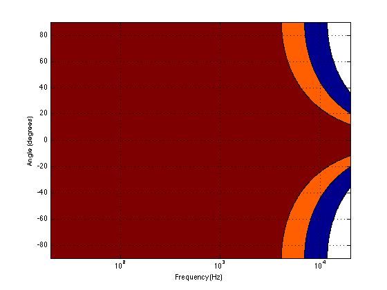
Normally, however, you do not make a loudspeaker out of either a woofer or a tweeter – you put them together to cover the entire frequency range. So, let’s look at a plot of that behaviour. I’ve put together our two pistons using a 4th-order Linkwitz-Riley crossover at 1.5 kHz. I have also not included any weirdness caused by the separation of the drivers in space. This is theoretical world where the tweeter and the woofer are in the same place – an impossible coaxial loudspeaker.

In Figure 5 you can see the effects of the woofer’s directivity starting to beam below the crossover, and then the tweeter takes over and spreads the radiation wide again before it also narrows.
So what?
Why should you care about understanding the plot in Figure 5? Well, remember that the narrower the radiation of a loudspeaker, the closer the sound will appear to be to you. This means that, for the imaginary loudspeaker shown in Figure 5, if you’re playing a recording without additional reverberation, the low frequency stuff will sound far away (the same distance as the loudspeakers), So will a narrow band between 3 kHz and 4 kHz (where the tweeter pulls the radiation wider). However, the materials in the band around 700 Hz – 2 kHz and in the band above 7 kHz will sound much closer to you.
Another way to express this is to show a graph of the resulting level of the reverberant energy in the listening room relative to the direct sound, an example of which is shown in Figure 6. (This is a plot copied from “Acoustics and Psychoacoustics” by David Howard and Jamie Angus).

This shows a slightly different loudspeaker with a crossover just under 3 kHz. This is easy to see in the plot, since it’s where the tweeter starts putting more sound into the room, thus increasing the amount of reverberant energy.
What does all of this mean? Well, if we simplify a little, it means that things like voices will pull apart in terms of apparent distance. Consonant sounds like “s” and “t” will appear to be closer than vowels like “ooh”.
So, whaddya gonna do about it?
All of this is why one of the really important concerns of the acoustical engineers at Bang & Olufsen is the directivity of the loudspeakers. In a previous posting, I mentioned this a little – but then it was with regards to identifying issues related to diffraction. In that case, directivity is more of a method of identifying a basic problem. In this posting, however, I’m talking about a fundamental goal in the acoustical design of the loudspeaker.
For example, take a look at Figures 7 and 8 and compare them to Figure 9. It’s important to note here that these three plots show the directivities of three different loudspeakers with respect to their on-axis response. The way this is done is to measure the on-axis magnitude response, and call that the reference. Then you measure the magnitude response at a different angle, and then calculate the difference between that and the reference. In essence, you’re pretending that the on-axis response is flat. This is not to be interpreted that the three loudspeakers shown here have the same on-axis response. They don’t. Each is normalised to its own on-axis response. So we’re only considering how the loudspeaker compares to itself.

Figure 7, above, shows the directivity behaviour of a commercially-available 3-way loudspeaker (not from Bang & Olufsen). You can see that the woofer is increasingly beaming (the directivity gets narrow) up to the 3 – 5 kHz area. The midrange is beaming up above 10 kHz or so. So, a full band signal will sound distant in the low end, in the 6-7 kHz range and around 15 kHz. By comparison, signals at 2-4 kHz and 10-15 kHz will sound quite close.

Figure 8, above, shows the directivity behaviour of a 3-way loudspeaker we made as a rough prototype. This is just a woofer, midrange and tweeter, each in its own MDF box – nothing fancy – except that the tweeter box is not as wide as the midrange box which is narrower than the woofer box. You can see that the woofer is beaming (the directivity gets narrow) just above 1 kHz – although it has a very weird wide directivity at around 650 Hz for some reason. The midrange is beaming up from 5kHz to 10 kHz, and then the tweeter gets wide. So, this loudspeaker will have the same problem as the commercial loudspeaker
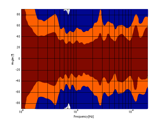
As you can see, the loudspeaker with the directivity shown in Figure 9 (the BeoLab 5) is much more constant as you change frequency (in other words, the lines are more parallel). It’s not perfect, but it’s a lot better than the other two – assuming that constant directivity is your goal. You can also see that the level of the signal that is within 1 dB of the on-axis response is quite wide compared with the loudspeakers in Figures 7 and 8. The loudspeaker in Figure 7 not only beams in the high frequencies, but also has some strange “lobes” where things are louder off-axis than they are on-axis (the red lines).
When you read B&O’s marketing materials about the reason why we use Acoustic Lenses in our loudspeakers, the main message is that it’s designed to spread the sound – especially the high frequencies – wider than a normal tweeter, so that everyone on the sofa can hear the high hat. This is true. However, if you ask one of the acoustical engineers who worked on the project, they’ll tell you that the real reason is to maintain constant directivity as well as possible in order to ensure that the direct-to-reverberant ratio in your listening room does not vary with frequency. However, that’s a difficult concept to explain in 1 or 2 sentences, so you won’t hear it mentioned often. However, if you read this paper (which was published just after the release of the BeoLab 5), for example, you’ll see that it was part of the original thinking behind the engineers on the project.
Addendum 1.
I’ve been thinking more about this since I wrote it. One thing that I realised that I should add was to draw a comparison to timbre. When you listen to music on your loudspeakers in your living room, in a best-case scenario, you hear the same timbral balance that the recording engineer and the mastering engineer heard when they worked on the recording. In theory, you should not hear more bass or less midrange or more treble than they heard. The directivity of the loudspeaker has a similar influence – but on the spatial performance of the loudspeakers instead of the timbral performance. You want a loudspeaker that doesn’t alter the relative apparent distances to sources in the mix – just like you don’t want the loudspeakers to alter the timbre by delivering too much high frequency content.
Addendum 2.
One more thing… I made the plot below to help simplify the connection between directivity and Grover. Hope this helps.
