#72 in a series of articles about the technology behind Bang & Olufsen loudspeakers
After a previous posting, someone posted this as part of a comment:
“What I’ve been asking myself for a long time: how does a single driver manage to produce two or more frequencies (or a frequency range) at the exact same time? For example a singer singing while the guitar plays in the background. Could you try to explain how this works?”
So, this posting is an attempt to answer that question.
Adding signals together
Sound is a change of air pressure over time. That pressure is modulating on top of the day’s average barometric pressure – which is just a measurement of how closely the air particles around you are squeezed together. On a high-pressure day, the air is more densely packed – on a low pressure day, the air is less dense.
When you make a sound, you make slight variations in that pressure – so, for example, when a woofer moves out of a loudspeaker enclosure (a fancy name for “box”) then it pushes the air particles in front of it, and they’re squeezed together, resulting in a compression wave that radiates away from the loudspeaker. When the woofer pulls into the enclosure, it pulls the air particles apart, and you get a rarefaction wave instead. (You can see an animation of this at this posting.)
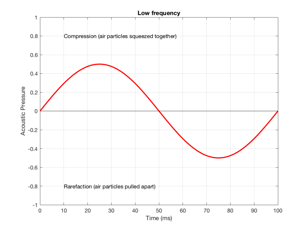
Let’s make a graph that shows a plot of the acoustic pressure changing over time. This is shown below in Figure 1. When this plot shows a positive number, it means that the air particles are being compressed more than normal. When it’s negative, then they’re being separated more than normal. Without getting into too many details, let’s just say that this is a low frequency. (If you want to get picky, then you’ll see that this is one cycle of a wave that takes 100 ms. Since there are 1000 ms in a second, then this must be a 10 Hertz signal, because 1000 / 100 = 10. That makes it a VERY low frequency by normal audio standards… )
Let’s also look at an example of a higher frequency, shown in Figure 2, below.
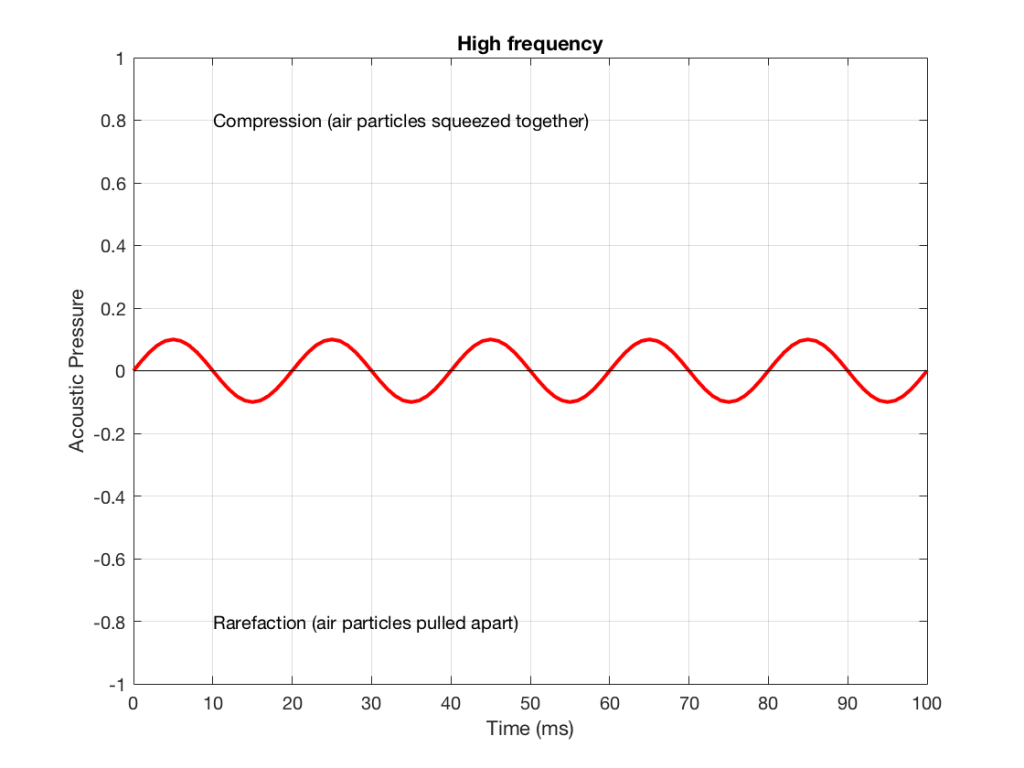
We can see that Figure 2 has a higher frequency signal, because it moves up and down more frequently. It has 5 cycles (5 ‘ups’ and ‘downs’) in the same amount of time that it took the wave in Figure 1 to have 1 cycle – therefore it is 5 times the frequency (and therefore, if you’re being picky, 50 Hz – which, by audio standards, is also a very low frequency, but this is just an example…)
Ignoring that ACTUAL frequencies that are plotted there, let’s pretend for a moment that the low frequency (Figure 1) came from a bass guitar and the higher frequency (Figure 2) came from a singer. If we took those two signals and put them into a mixing console, what does the result look like?
Well, we take the instantaneous value of the signal at one moment in time and add it to the instantaneous value of the other signal at the same time. Let’s do that.
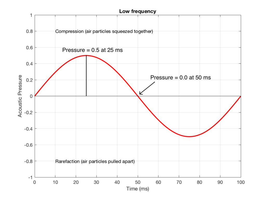
Figure 3 shows the same signal as in Figure 1, but I’ve pointed out the values at two moments in time – at 25 ms and at 50 ms. So, for example, you can see there that, at 25 ms, the value is 0.5 – whatever that means…
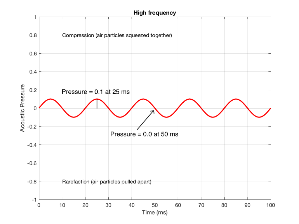
Figure 4 shows the same signal as in Figure 2, but I’ve pointed out the values at two same moments in time – at 25 ms and at 50 ms. So, for example, you can see there that, at 25 ms, the value is 0.1 – whatever that means.
We take the value at 25 ms from each of the two signals (0.5 and 0.1) and add them together to get 0.6. This is the value of the signal at the output of the mixer at 25 ms. At 50 ms, the mixer’s output will have a value of 0 (because 0+0 = 0). This is shown graphically below for all of the values of both plots from 0 ms to 100 ms.
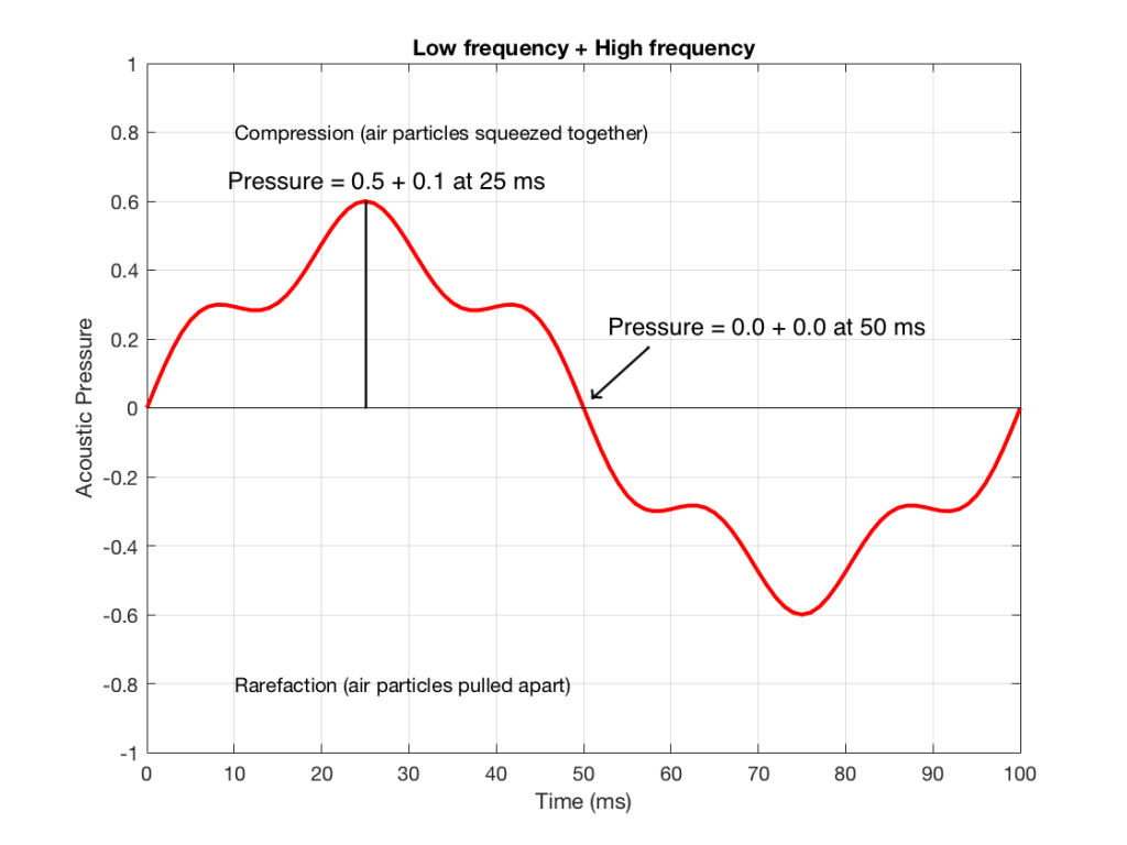
So, you can see in Figure 5 what the result will be. This signal contains both the low frequency, shown in Figure 1 and the higher frequency shown in Figure 2. If we send this combined signal to a loudspeaker, then both signals will get reproduced.
One interesting thing to note is that this mixing can also be done in the air. If a bass guitar and a singer are performing a song together, live, then the bass is pushing and pulling the molecules at the same time that the singer’s voice does. So, if at 25 ms, the bass pushes the molecules with a value of 0.5 (whatever that means) and the singer pushes the molecules with a value of 0.1, then your eardrum will be pushed in with a value of 0.6. So, the summation of the pressure signals happens in the air, just like it does as voltages or voltage measurements in the mixing console.
Splitting signals apart
Typically, however, a loudspeaker is comprised of more than one driver – for example, a woofer (for the low frequencies) and a tweeter (for the high frequencies). (Of course, some loudspeakers have more than two drivers, but we’re keeping things simple today…)
So, what we do there is to put the total signal, shown in Figure 5, and send it to two circuits that change how loud things are, depending on their frequency. One circuit is called a “low pass filter” because it allows low frequencies to pass through it unchanged, but it reduces the level of higher frequencies. The other circuit is called a “high pass filter” because it allows the high frequencies to pass through it unchanged, but it reduces the level of the lower frequencies. (we won’t talk about how those circuits do that in this posting…)
We can plot the two characteristics of these two circuits – an example of which is shown in Figure 6.
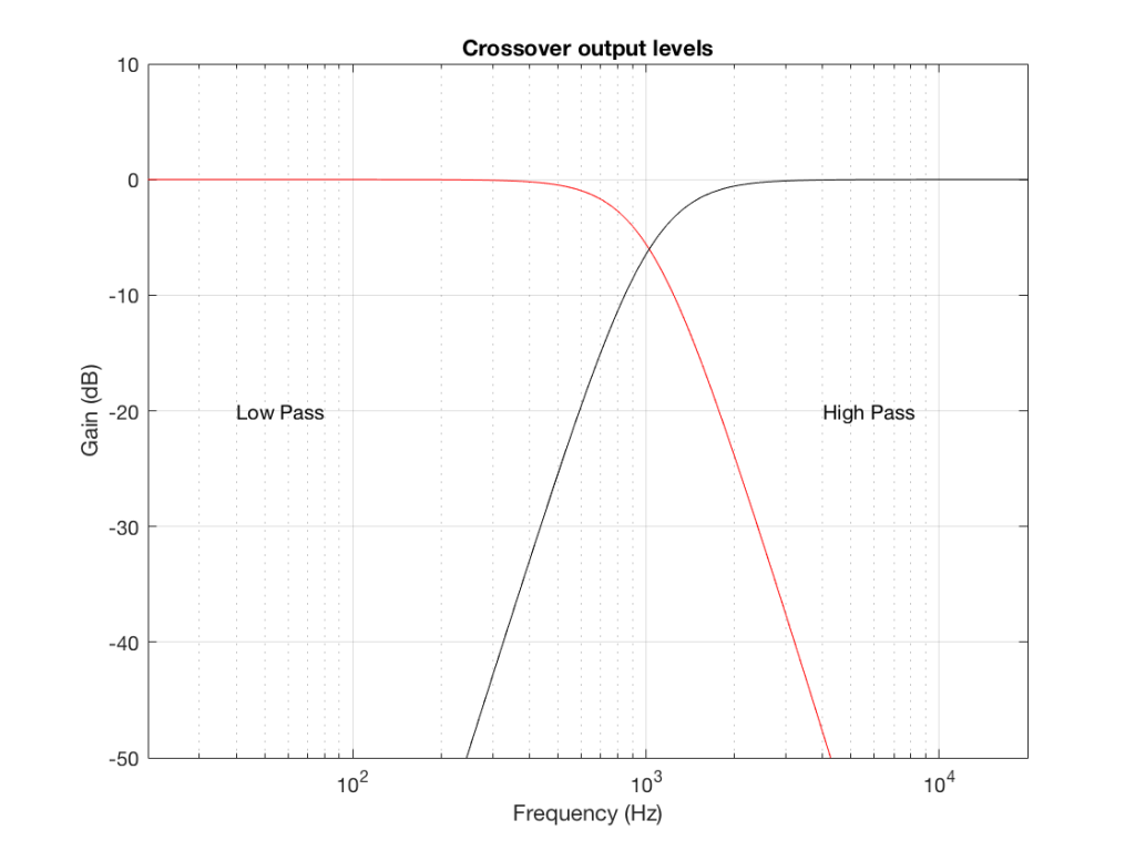
IF we send a signal like the one in Figure 5 to a crossover that happens to have a crossover frequency that is between the two frequencies it contains, then the signal will be split into two – one output containing mostly low-frequency components, and the other one containing mostly high-frequency components. Examples of these are shown below.
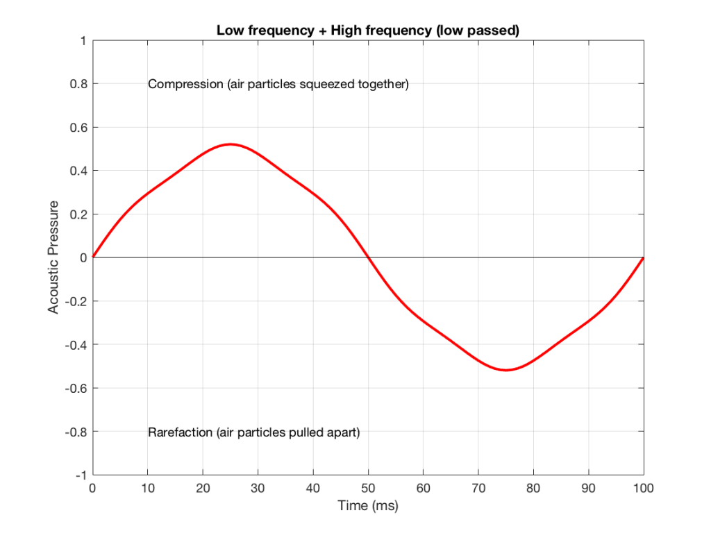
NB: Of course, everything I’ve shown here are just examples to make the concept intuitive. The crossover shown in Figure 6 would not work the way I’ve shown it in Figures 7 and 8 because the crossover frequency is too high compared to the 10 Hz and 50 Hz waves that I used in the example. So, please do not make comments talking about how I chose the wrong crossover frequency…