I’m originally from Newfoundland – one of the few places in the world with a 1/2-hour time zone. So, when it’s 10:00 a.m. in Montreal, it’s 11:30 a.m. in St. John’s – my home town. This meant that, when I was a kid 40 years ago, and we would call our relatives in Toronto or Germany to wish them a Merry Christmas, there were two questions that you could always rely on being asked: (1) what’s the weather like there? and (2) what time is it there?
These days, I have a similar problem that is well-described by “Segal’s Law“. My iPhone and my wristwatch (an old analogue one with hands that go around pointing at the floor and the fridge…) are never synchronised… This is because of two things: (1) I probably did a bad job of setting my watch and (more importantly) (2) my watch runs just a little bit slowly…
So, let’s say, for example, that I set my watch to be EXACTLY in sync with my phone on a Monday morning at 9:00 a.m. As the week goes by, my iPhone and my watch drift apart, and, just for the sake of argument let’s say that, one week later, when my iPhone turns over to 9:00 a.m. on Monday morning, my wristwatch turns over to 8:59 a.m. So, I lose 1 minute per week on my watch.
(It’s pretty safe to assume that my iPhone is also not perfect – but it’s different because, every once in a while, it compares its internal clock with another, more accurate clock somewhere else via a connection across the Internet (which, we will assume, for the purposes of this discussion, works).)
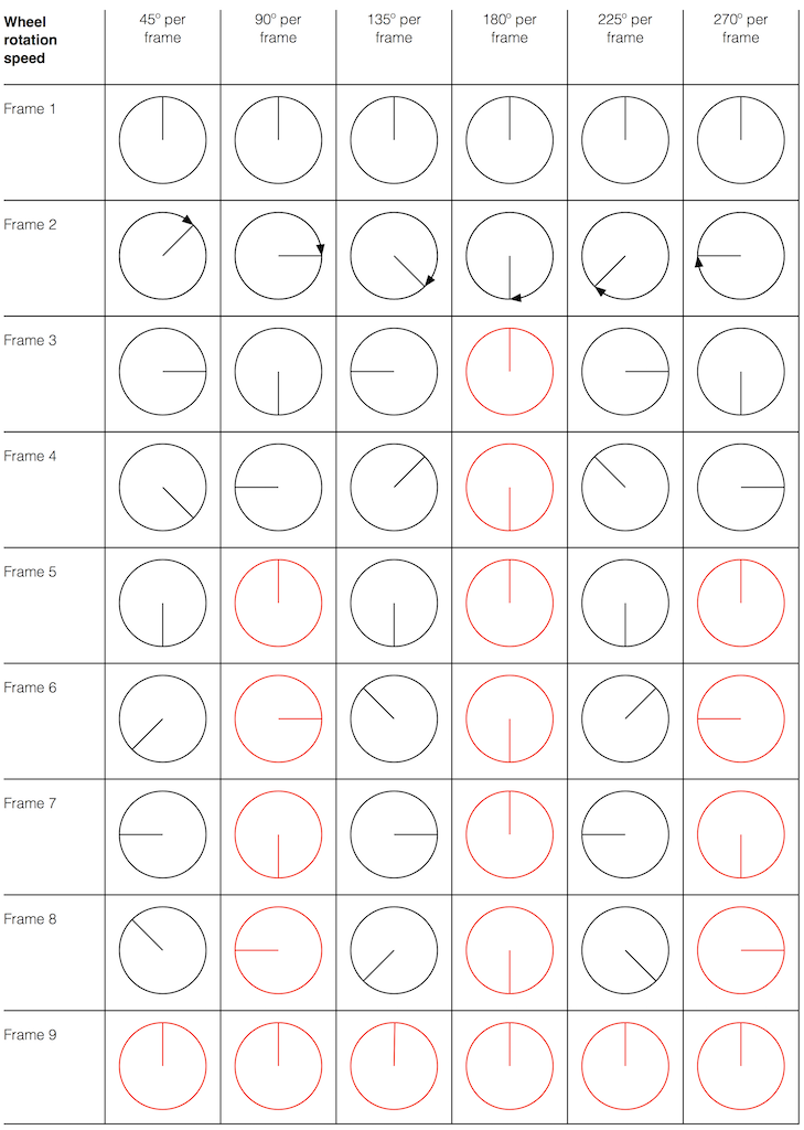
Let’s consider this from a strange point of view. Let’s assume that
- I’m checking the time on my watch every minute, on the minute
- someone else is “fixing” my watch every week so that it’s correct at 9:00 a.m. on Mondays. They do this by adjusting the watch to the correct time 30 seconds before the iPhone says it’s 9:00 a.m.
- I don’t know that they’re doing this for me…
If we think about this from my perspective, I’ll live in a strange world where 8:59 on Mondays never exists. This is because at 8:58 and 30 seconds (on my watch), my friend re-sets the time to 8:59 and 30 seconds (while I’m not looking) to synchronise with the iPhone…
IF my watch was running fast – say, gaining one minute each week, then I would live in a different strange universe where 9:00 happens twice every Monday morning…
The basic problem here is that we have two clocks that do not run at the same rate – but they are expected to do so. So, we synchronise them regularly (in the above example, on Monday mornings at 9:00) – but between those synchronisation events, they drift apart in time.
So what?
The example above is very, very similar to the way a digital audio streaming system works – especially if you’re using a wireless connection between the transmitting device and a receiver.
Lets say that you’re playing a sound file that was recorded at 44.1 kHz and streaming it wirelessly to a receiver. I’m trying to be as generic as possible here, but I could be talking about a Bluetooth connection to a pair of headphones or a WiFi connection via DLNA to a device connected to a pair of loudspeakers, for example…
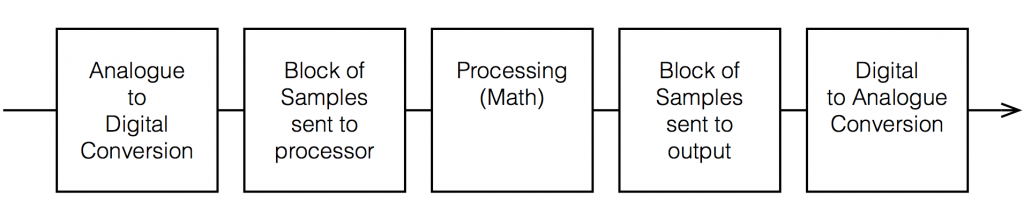
It is not unusual with such a connection for the transmitter to collect up a block of audio samples – say, 64 of them – and send them to the receiver’s input buffer. The receiver then pulls those samples out, one by one, and (eventually) sends them to a digital-to-analogue converter that produces a signal that (eventually) comes out as an audio signal. Then, 64/44100’ths of a second later (64 samples later) the transmitter sends another block, and so on and so on until the song ends.
This system works well if the clock inside the transmitter and the clock inside the receiver are perfectly synchronised. We can even be a little generous and say that they can drift apart a little – but not so much that we either run out of samples to play (because the receiver is playing them out faster than they’re coming in from the transmitter) or that we have samples left over to play when the next block comes in (because the receiver is playing them out slower than they’re coming in from the transmitter).
Dealing with this problem the right way
The right way to deal with this issue is for the receiver to always be checking what time it thinks it is when the block arrives from the transmitter. If the block arrives a little early, then the receiver should think “hmmmm, my clock is going too slowly – I’ll speed it up a bit”. If the block arrives a little late, then the receiver should adjust its clock to go a little slower.
So, in this case, the receiver has a basic, nominal speed for its internal clock – but it’s constantly adjusting it to be faster and slower to try and match the clock of the transmitter – but it can only do this adjustment at the block rate – the frequency at which the blocks of samples arrive, which is dependent on the block length (how many samples are in each block) and the sampling rate (how many samples per second). (Of course, this can result in “jitter and wander” problems if you’re not careful (I won’t talk about this here…) – so you have to pay a little attention to how quickly you’re adjusting your clock rate… but that’s “just” a matter of correct implementation.)
Dealing with this problem the wrong way
There is another way to deal with this problem, which, unfortunately, has measurable and possibly audible consequences. This implementation is basically the same as my original example, where I had a friend “fixing” my wristwatch once a week. You have a transmitter that sends blocks of samples to the receiver – and although these two devices should have exactly the same clock rate, they don’t.
Let’s say, for example, that the receiver is playing the samples faster than they’re being sent by the transmitter. This means that the two will slowly drift farther and farther apart until, eventually, the receiver will have to play a sample, but nothing has come in from the transmitter yet, so there’s no sample there to play. In this case, the receiver says “no problem, I’ll just play the last sample again, and the next block will come in while I’m doing that” – so it inserts an extra sample that is just a duplicate of the previous one.
If the receiver’s clock is going slower than the transmitter’s, then, as the two drift farther apart, we will get to a moment where the receiver will receive a new block of samples but it’s not done playing all of the samples in the previous block yet. In this event, it says “no problem, I’ll just leave that last sample out and move on to the next block to catch up” – so it skips a sample.
This is called a “Skip / Insert” strategy for dealing with clock synchronisation. It’s done by software and hardware engineers because it’s simple to implement, and, in many cases, a manufacturer can get away with this, since it is rarely audible for a couple of reasons.
Can this be measured?
The simple answer to this is “yes” – and it can be measured in a number of different ways. I’ll show one way below…
Can I hear it?
The honest answer to this question is “sometimes” – but it’s not as easy to detect as one might think. Of course, a skip/insert event (a duplicated sample or a dropped one) creates an artefact. However, the magnitude of this artefact relative to the “correct” signal is dependent on when it happens.
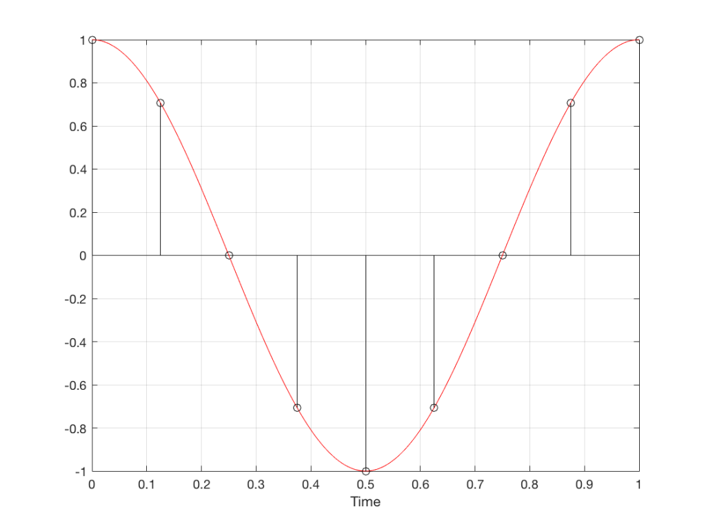
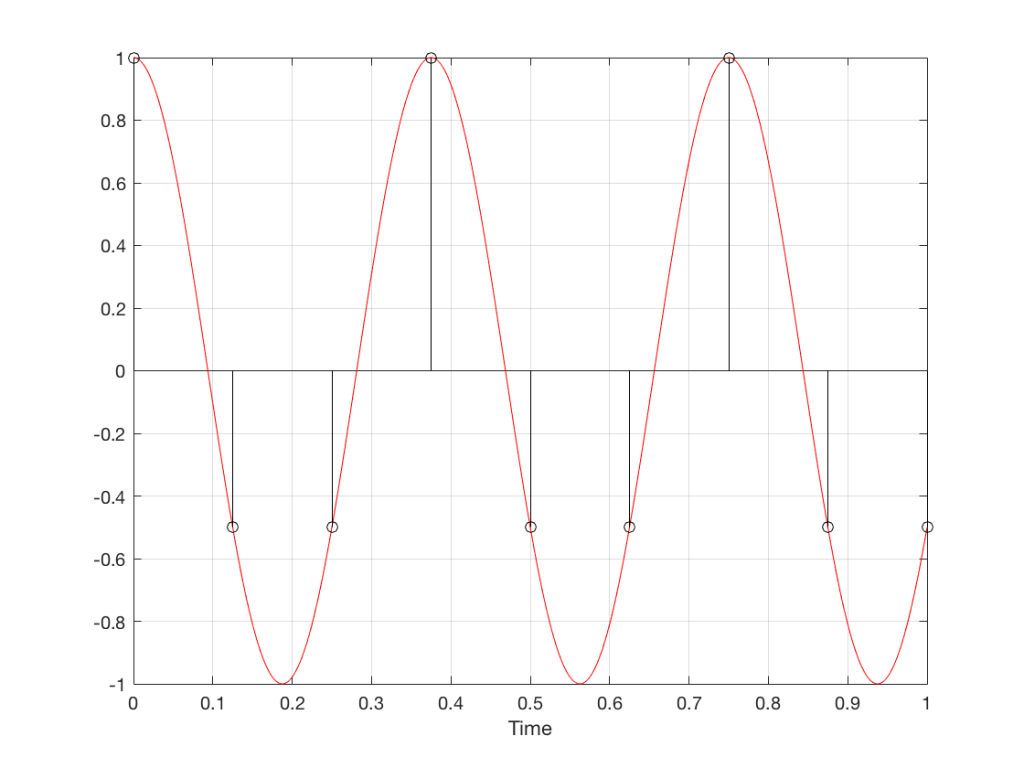
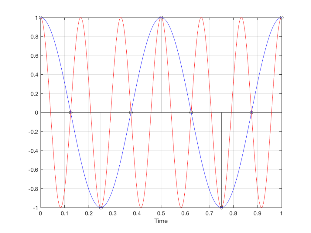
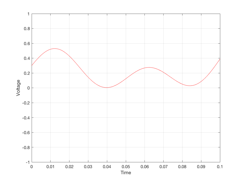
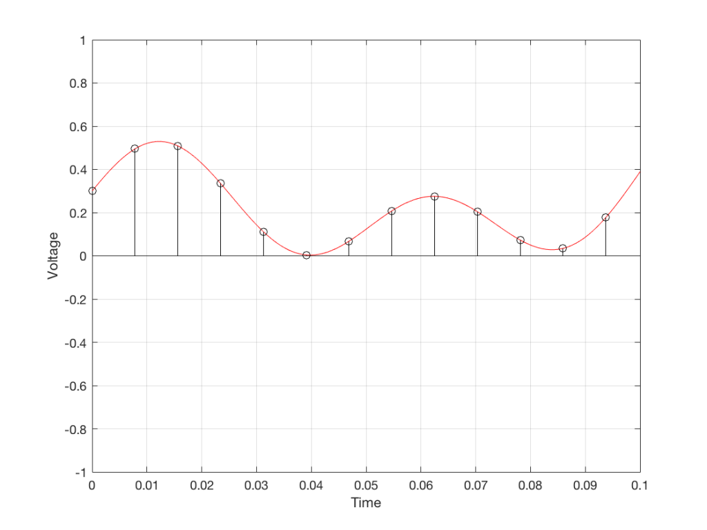
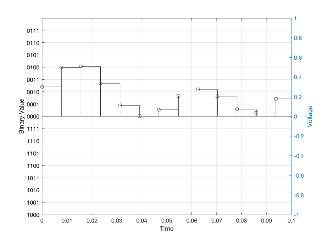
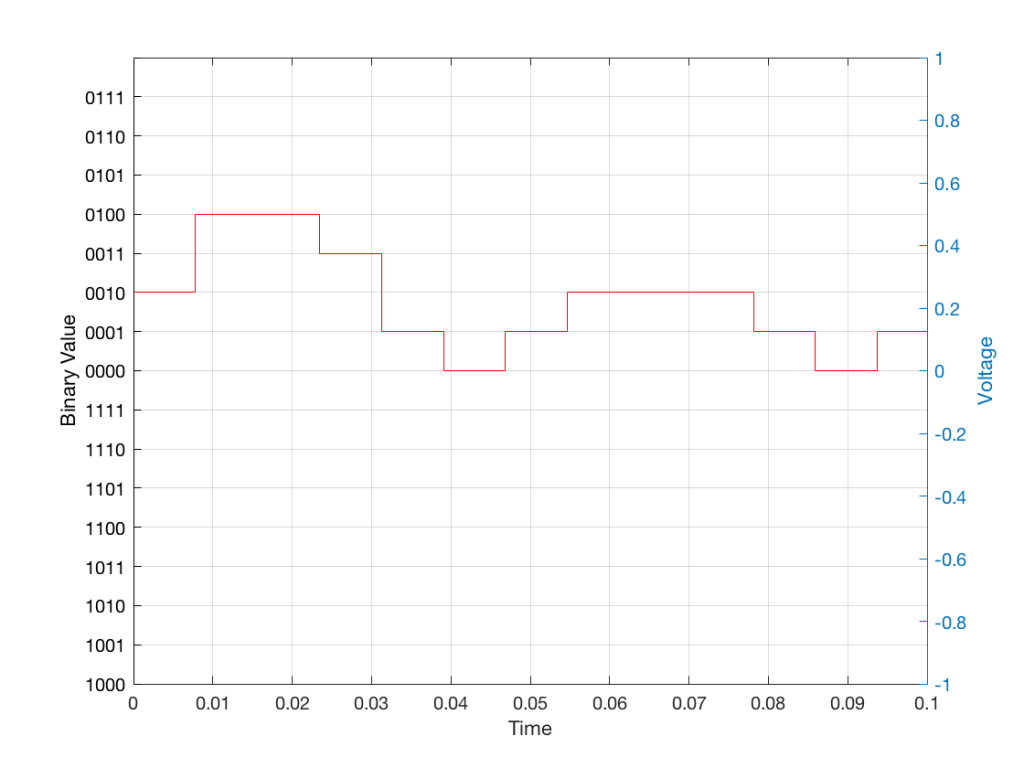
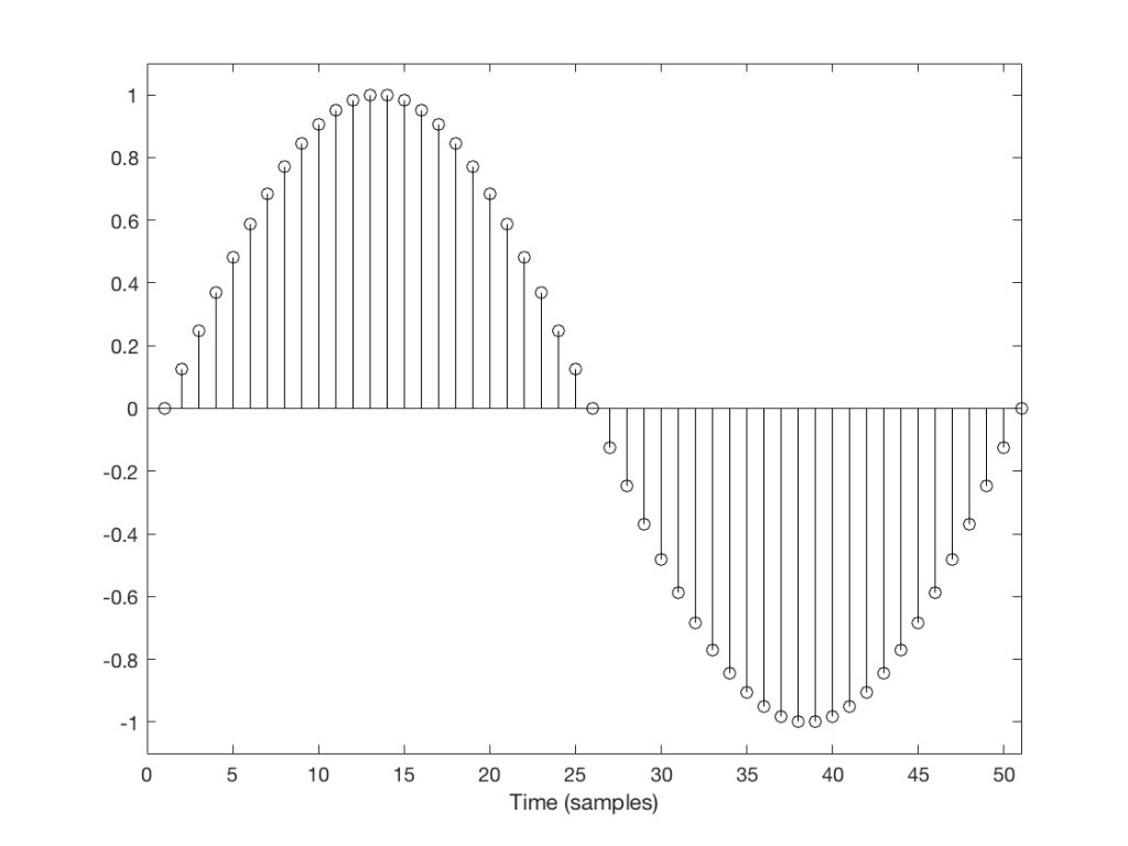
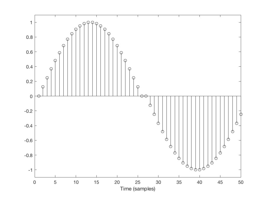
Let’s take a look at a couple of simple cases. We’ll “transmit” one period of a sine wave that should come out on the other side of the system looking like Figure 1.
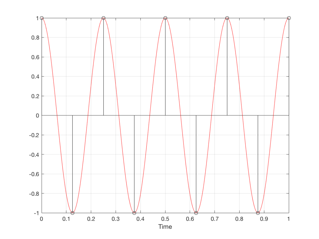
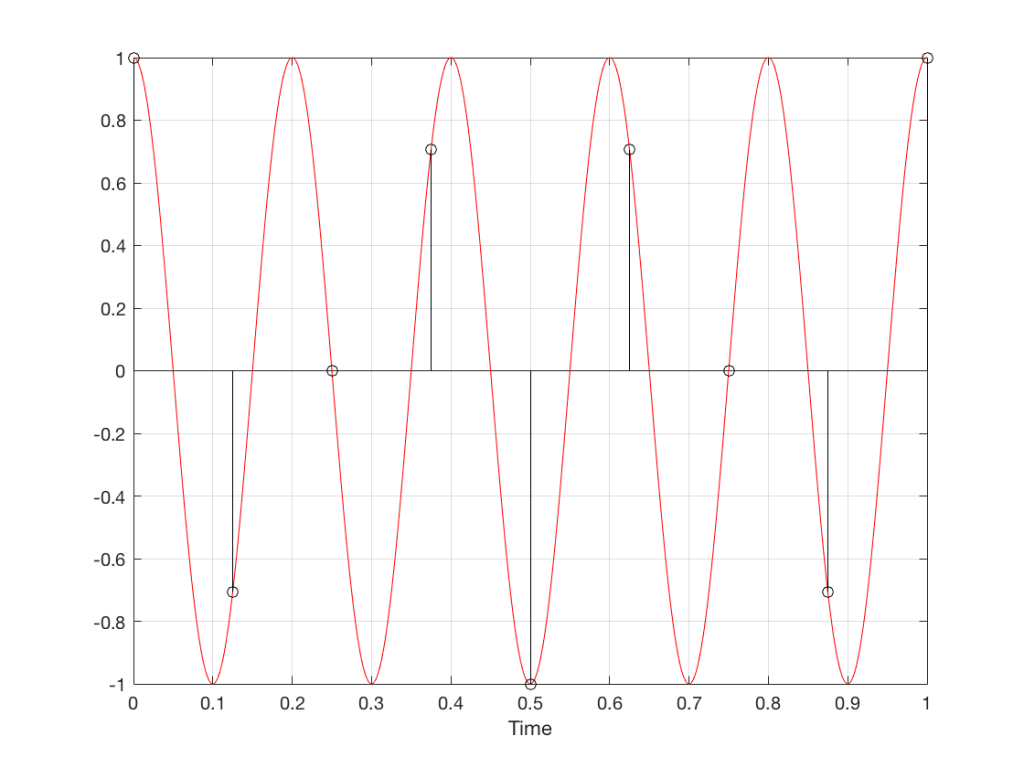
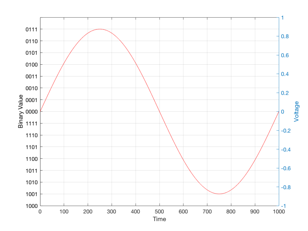
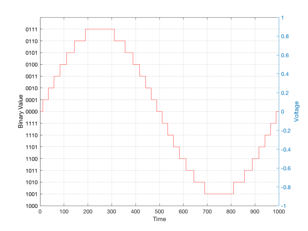
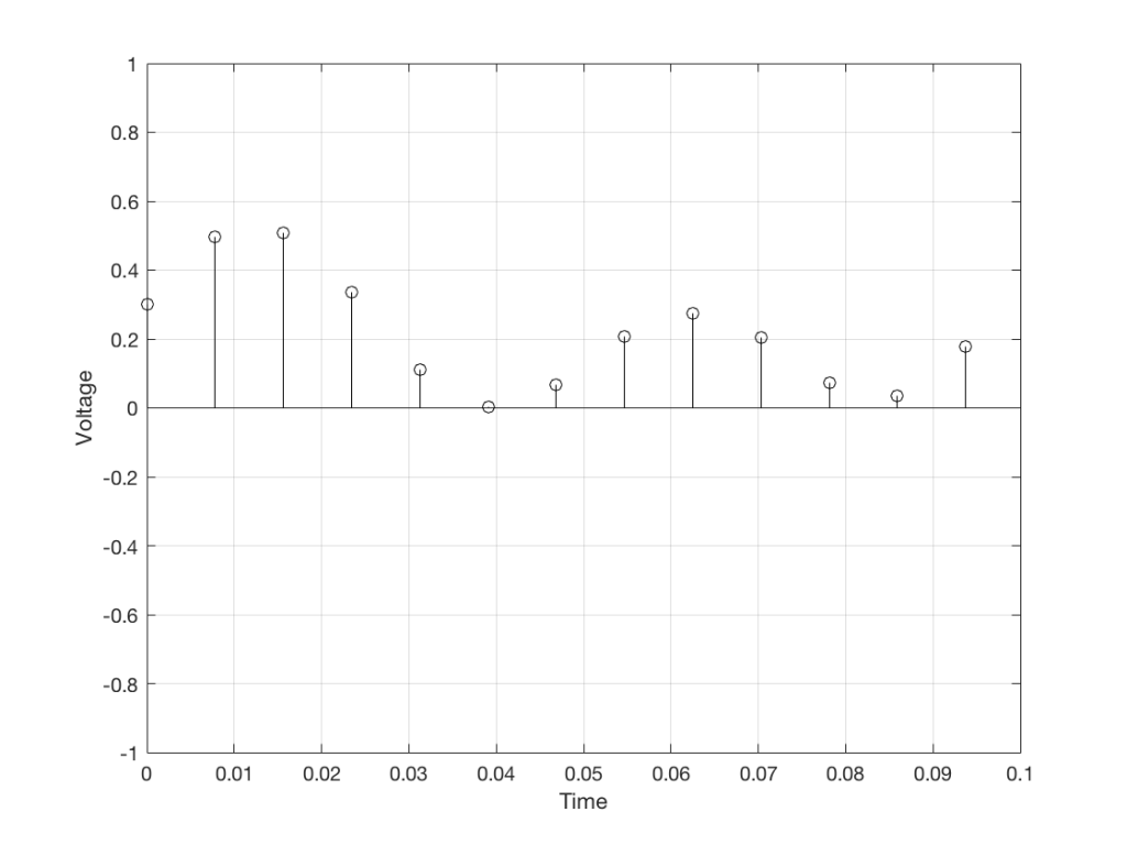
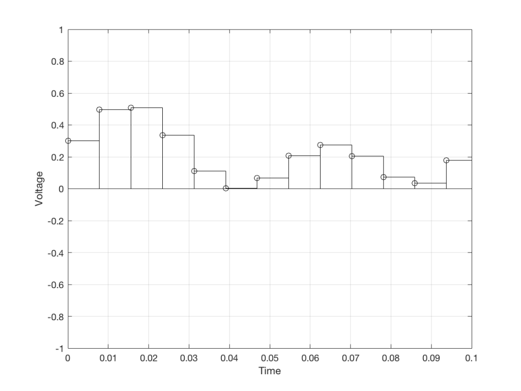
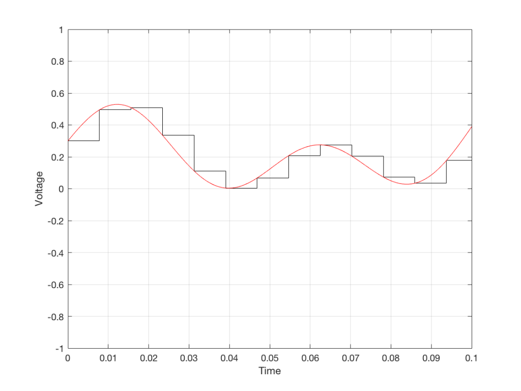
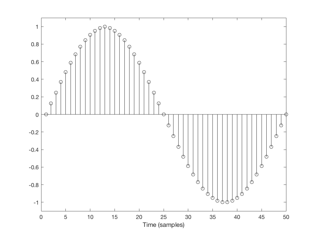
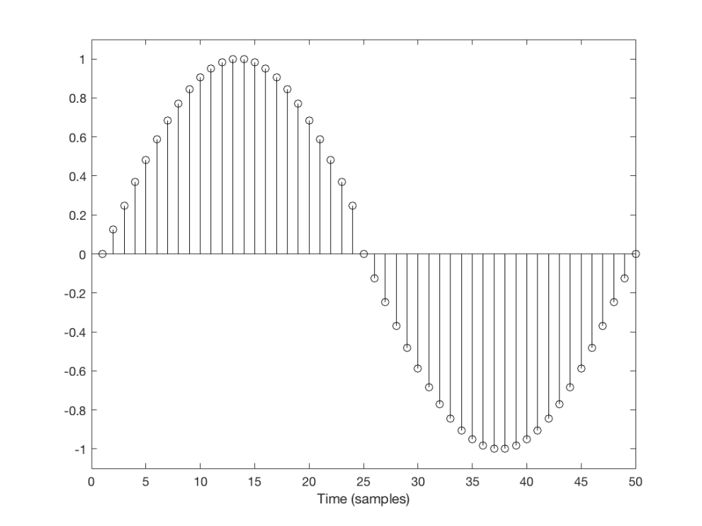
But what happens if we don’t get a block in time to keep outputting a signal? We insert a duplicate sample and hope that the block comes in before I have to send out another one. Examples of this are shown in Figures 2 and 3, below.

You’ll probably notice that it’s much easier to see which sample I duplicated in Figure 3 than in Figure 2. In Figure 3 it was sample number 26 that was duplicated. In Figure 2 it’s sample number 13.
The reason it’s easier to see the error in Figure 3 is that duplicating the sample causes an obvious change in the slope of the signal, whereas in Figure 2 it does not – the slope of the signal is 0, and by duplicating a sample, I am also making it 0 – but for a slightly longer time.
This does not mean that we did not generate an error. It just means that we’ll probably “get away with it” in the case of Figure 2, and we probably won’t in the case of Figure 3.
However, since the drifting of the two clocks (in the receiver and transmitter) are not dependent on the signal, there’s no way to know when this is going to happen.
And, of course, if this happens in the middle of a snare drum hit or a ssssinger sssstarting a word in a ssssong with the letter “s” – then we also won’t hear it because there’s so much going on (frequency-wise) that the artefact will be buried in the mess.
Also, since this clock drifting is usually not completely regular, the errors do not usually come in at a regular rate (although I’ve seen exceptions…). So, it’s not like you can listen for “a click every second” or “one per minute”. They happen when they happen – hopefully when you’re not listening and/or when the tune is busy enough to hide it.
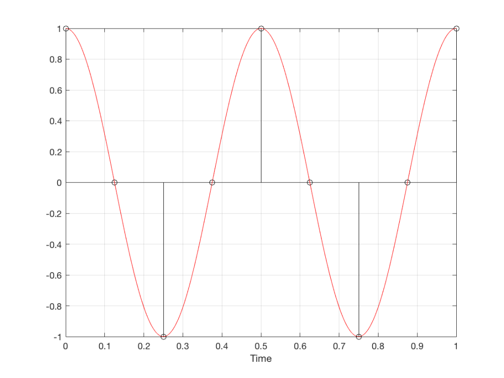
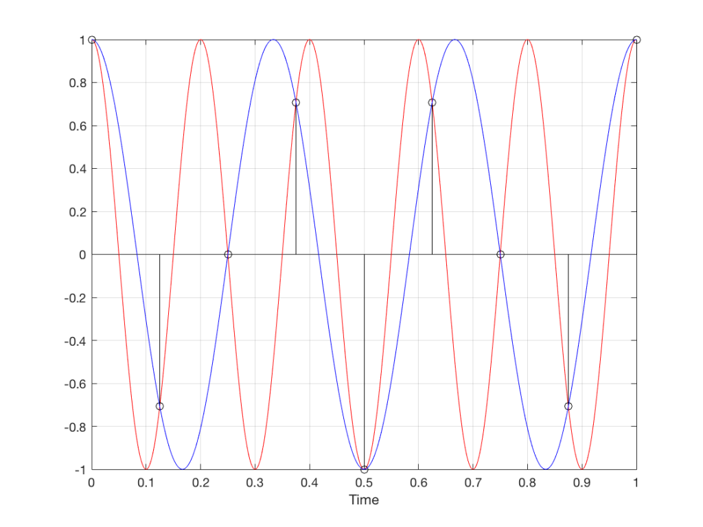
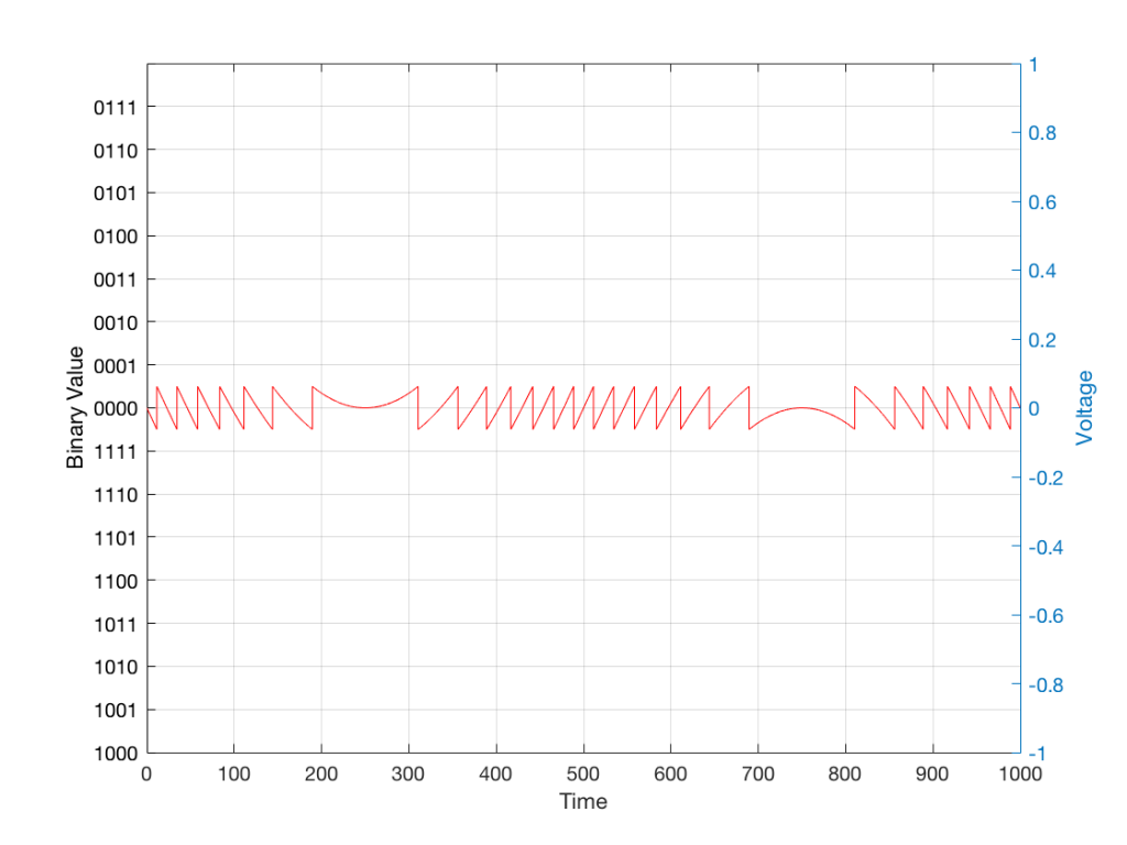
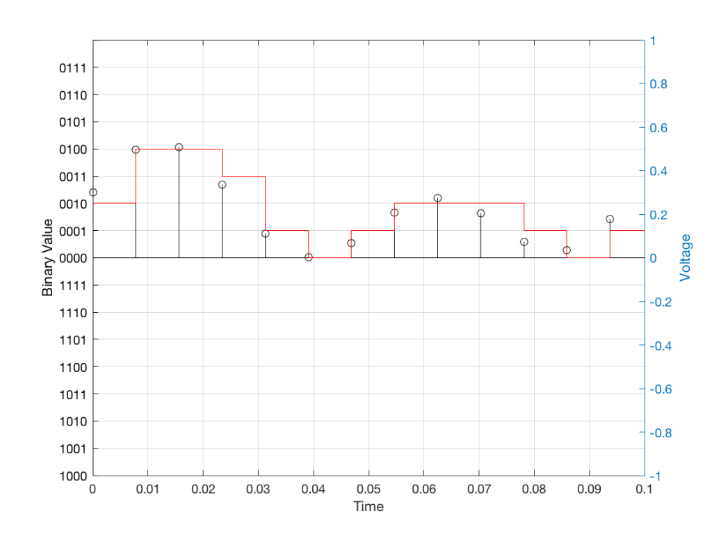
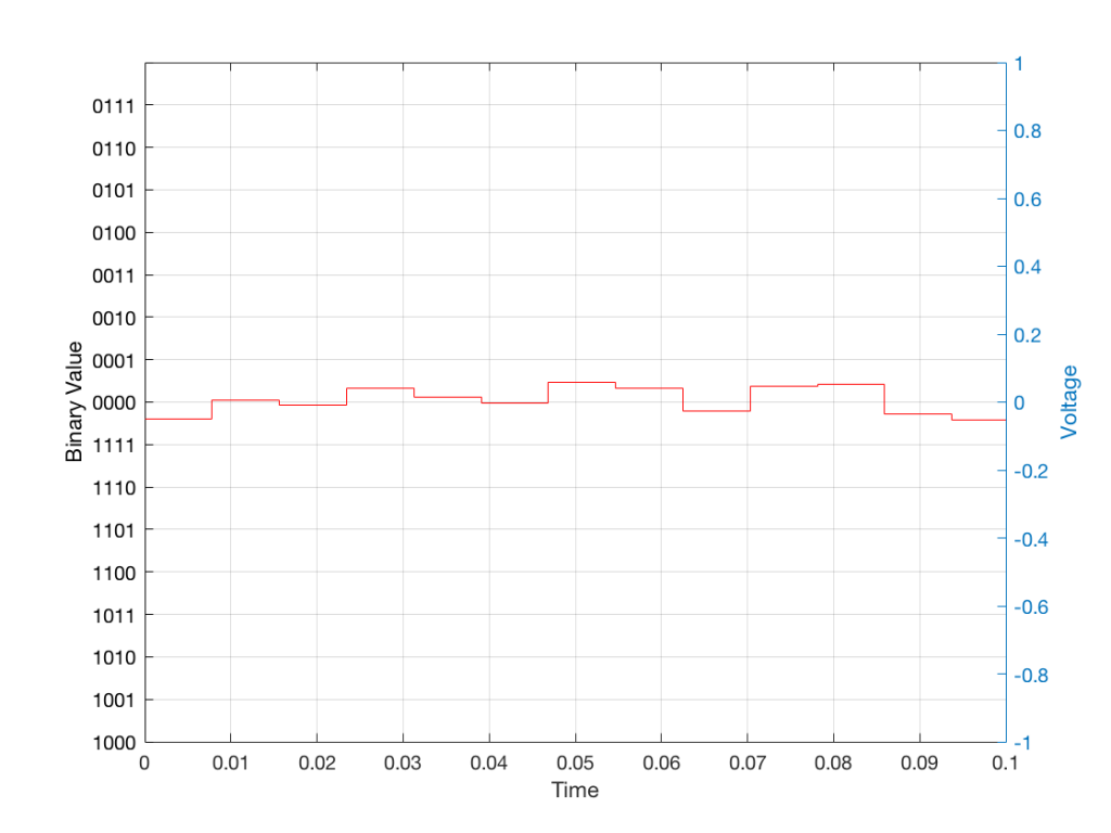
A skip event is similar to an insert, as you can see in the two examples in Figures 4 and 5.
Again, I’ve intentionally put in these two skips in places where they are least obvious (Figure 4) and most obvious (Figure 5).
The real world
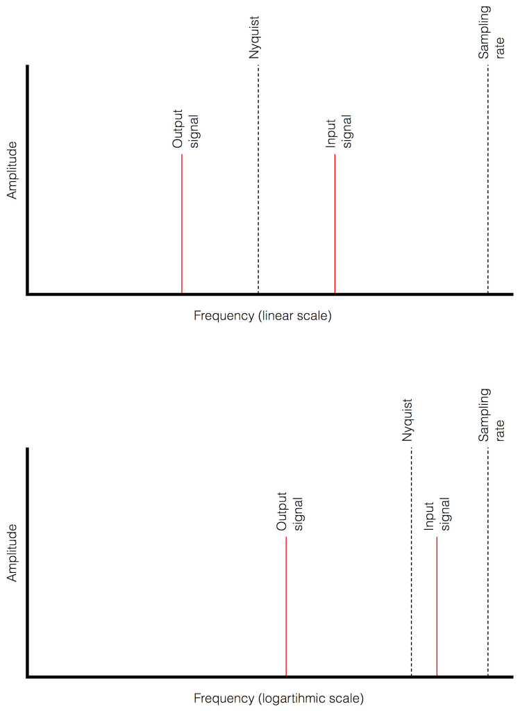
One of the tests that can be done on an audio system is to send a sinusoidal signal with a swept frequency through a system, capture the output, and then do a spectrogram of the result. In theory, if you see anything other than a single frequency at any one time at the output, then you know that something has happened to the signal. You would probably then need to go back and look at the output signal itself to start evaluating exactly what happened… This is a test that is used to evaluate one aspect of the performance of different sampling rate converters, for example, at this site.
Let’s take a sine sweep and run it through a system. The sweep goes up logarithmically in frequency from 20 Hz to about 90% of Nyquist (which would correspond to 20,000 Hz in a system running at 44.1 kHz) over 60 seconds and has a level of -1 dB FS. We’ll then capture the output in a system that is behaving perfectly and do a spectrogram of this, looking for artefacts down to some level below the signal level. (If you’re really geeky, you’ll know that this signal-to-error ratio is dependent on the window length of the FFT I’m using to create the spectrogram – but this is beyond our discussion today…).
An example of the output of a system that is behaving well is shown in Figure 6.
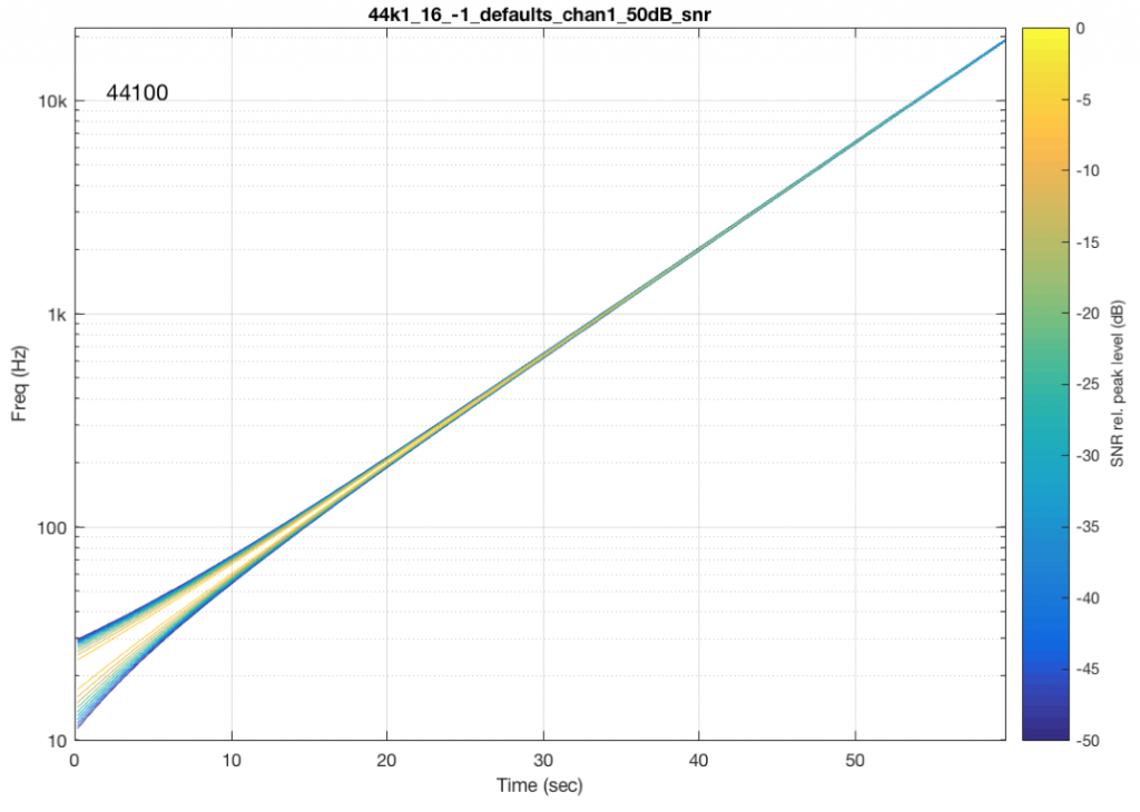
You may notice that the plot looks a little “wide” in the beginning. This is because the window length of the FFT I’m using to analyse the signal isn’t long enough to get a precise analysis of a low-frequency signal. So, this is an artefact of the analysis – not an error in the playback system.
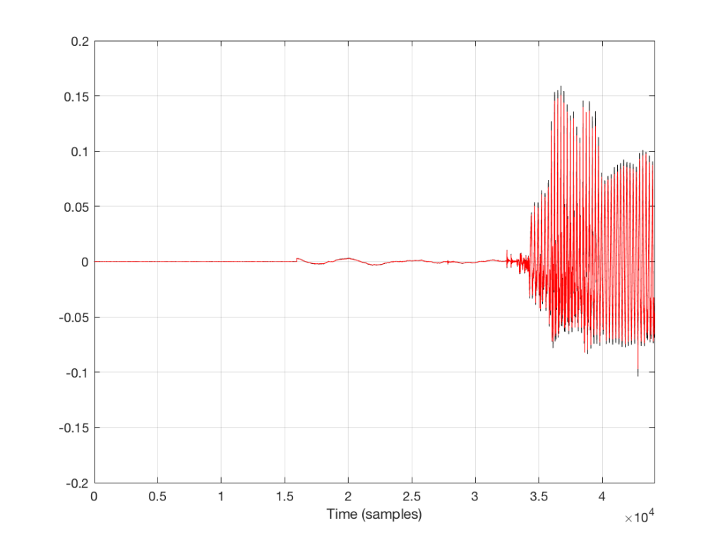
What happens if we have random skip/insert events in the system? This is shown in Figure 7.
The signal in Figure 7 was one that I created – I intentionally made skip/insert events at random times and applied them to my test signal.
There are two things to notice here. The first is that each event is visible as a vertical “spike” in the plot. This is because a skip/insert event will cause a short, wide-band “burst” that sounds like a click. However, the bandwidth of the click is dependent on when it happens relative to the signal. For example, the skip/insert events in Figure 2 and 4 would not create as much high-frequency energy as the ones in Figure 3 and 5. So, the bigger the effect on the slope of the signal, the more high frequency energy we’ll get in our “click” sound. Since the slope of a signal increases with frequency, then this also means that low-frequency signals will likely produce lower-bandwidth artefacts.
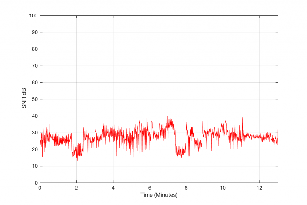
Now let’s look at the results from some real-world devices and systems that are commercially available.
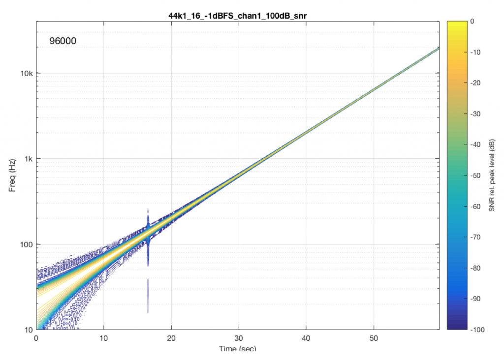
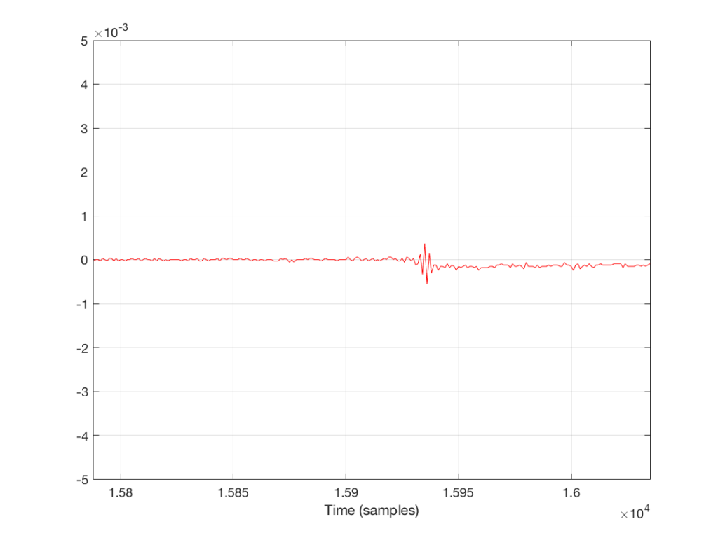
As you can see in Figure 8, there was one skip/insert event that happened during the 60 seconds I was running this test. Remember that the time that that event happened had nothing to do with the frequency it was playing. It just happens when it happens due to the relationship between the transmitter’s and the receiver’s clock speeds.
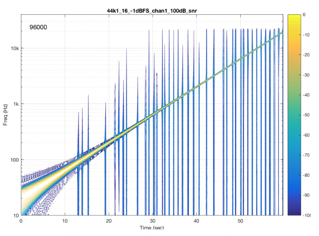
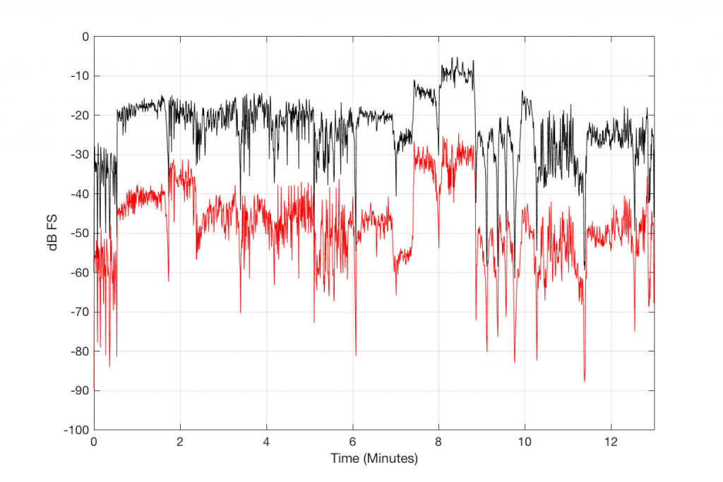
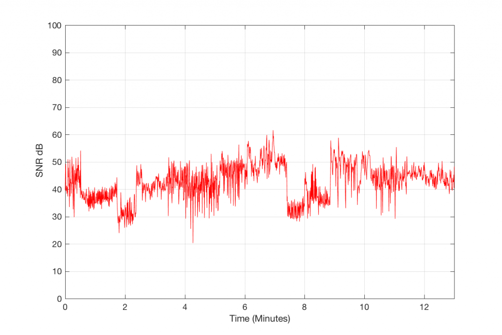
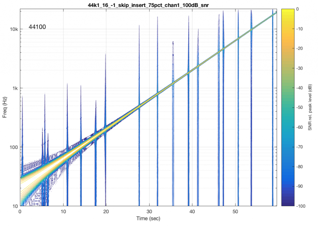
Figure 9 shows the results from a different system/device that obviously uses a skip/insert strategy to deal with clock synchronisation problems. It also obviously has some serious clock issues, since it has to correct on the order of approximately once a second…
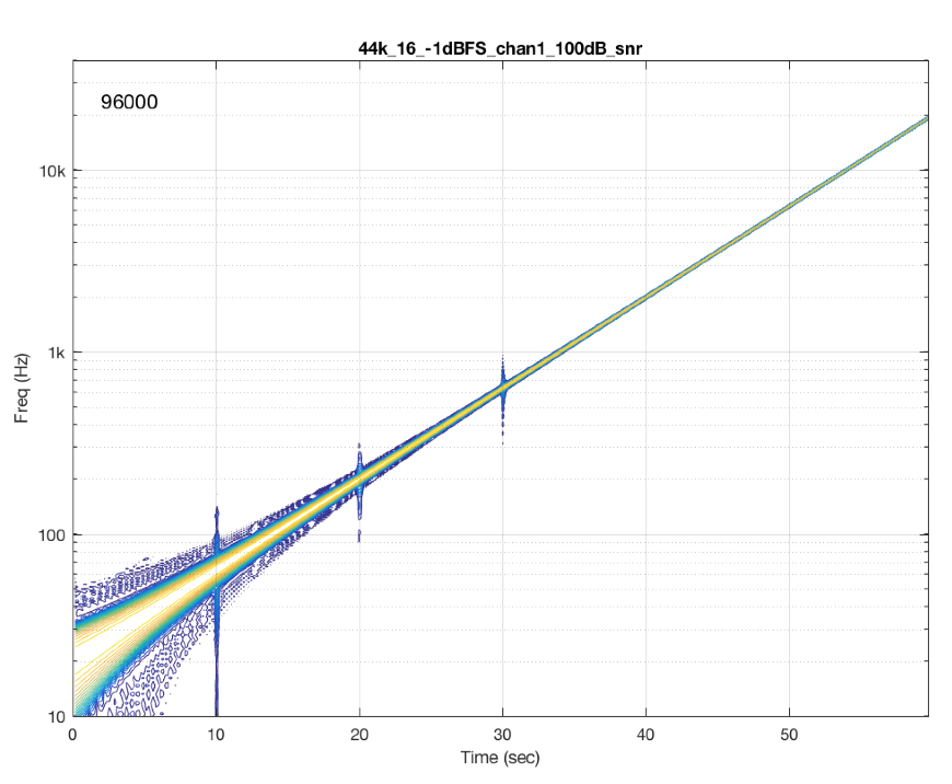
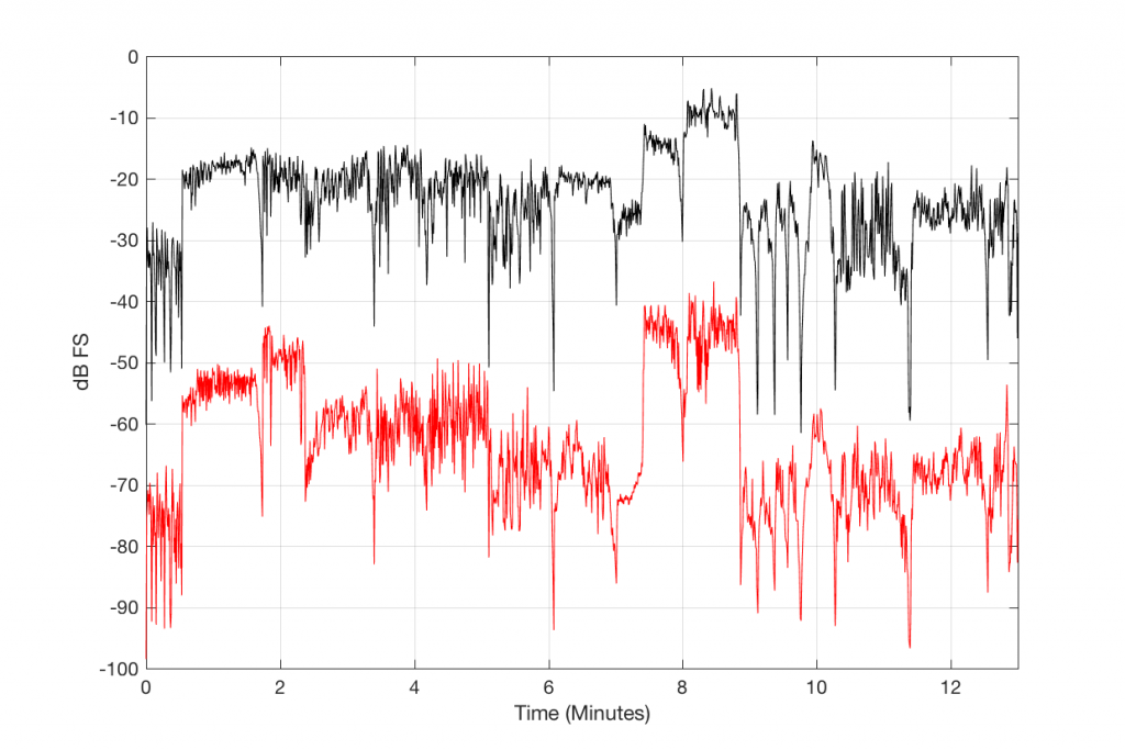
Figure 10 shows the results from a different system/device that uses a skip/insert strategy – but appears to do so at scheduled intervals. In this case, there is a high probability of getting a skip/insert event every 10 seconds with the counter starting at the instant I starting hearing the music.
Addendum 1
Inquisitive readers may be asking why it is that, although I’m doing an analysis down to -101 dB FS (100 dB below the signal level of -1 dB FS), you can’t see the effects of the dither noise floor in my original 16-bit file (which is normally assumed to be at -93 dB FS). This is because the -93 dB FS estimate of a dither signal assumes that you are looking at the total energy from the entire frequency band. The spectrograms above are based on FFT’s that split up the total frequency band into “slices” (called frequency bins) – and the total energy in each of these bins is less than the total energy in all of them (one person clapping is not as loud as 1000 people clapping at the same time…). If we wanted to see the dither noise, I would have had to set my analysis to go down approximately 30 dB lower – but the actual value for this is dependent on the relationship between the sampling rate, the window length of the FFT’s, and the windowing function that I’m using.
Addendum 2
Do not bother contacting me to ask which “commercially-available system/device” I measured and in which I found these errors. I’m not doing this to get anyone in trouble. I’m just doing this to try to illustrate common errors that I see often when I evaluate and test audio devices.
An besides, it would not be fair for me to rat on specific companies, systems, or devices, since, in some cases, these errors may have already been fixed with a firmware update, meaning that “naming names” would be irrelevant and unnecessarily detrimental.
But, I will say that I see this problem often. A rough estimate is that I would see errors like this on roughly half of the commercially-available devices and systems I test. It can also be sneaky, as we saw in Figures 8 and 10. Sometimes you get one of these clicks only once in a minute. So, if you do a 10-second measurement to test if your wireless audio receiver is “bit accurate” – the answer can be “yes” – but if you keep measuring for 1 or 2 minutes, you find out the answer is “no”…
Addendum 3
If it helps, I could have used the example of a leap year instead of two clocks at the beginning. The reason we have a February 29 every 4 years is that our calendar “runs” a little faster than the time it takes us to get around the sun (because a “year” is actually 365.25 days long…). So, every 4 years we have to “insert” a day to put the two clocks back in sync.
Also, since a “year” is not exactly 365.25 days long, we also have the occasional “leap second” as well. But most people don’t notice this, since it’s rarely useful as an excuse when you’ve missed a meeting…