Reminder: This is still just the lead-up to the real topic of this series. However, we have to get some basics out of the way first…
In the last posting, I talked about digital audio (more accurately, Linear Pulse Code Modulation or LPCM digital audio) is basically just a string of stored measurements of the electrical voltage that is analogous to the audio signal, which is a change in pressure over time…
For now, we’ll say that each measurement is rounded off to the nearest possible “tick” on the ruler that we’re using to measure the voltage. That rounding results in an error. However, (assuming that everything is working correctly) that error can never be bigger than 1/2 of a “step”. Therefore, in order to reduce the amount of error, we need to increase the number of ticks on the ruler.
Now we have to introduce a new word. If we really had a ruler, we could talk about whether the ticks are 1 mm apart – or 1/16″ – or whatever. We talk about the resolution of the ruler in terms of distance between ticks. However, if we are going to be more general, we can talk about the distance between two ticks being one “quantum” – a fancy word for the smallest step size on the ruler.
So, when you’re “rounding off to the nearest value” you are “quantising” the measurement (or “quantizing” it, if you live in Noah Webster’s country and therefore you harbor the belief that wordz should be spelled like they sound – and therefore the world needz more zees). This also means that the amount of error that you get as a result of that “rounding off” is called “quantisation error“.
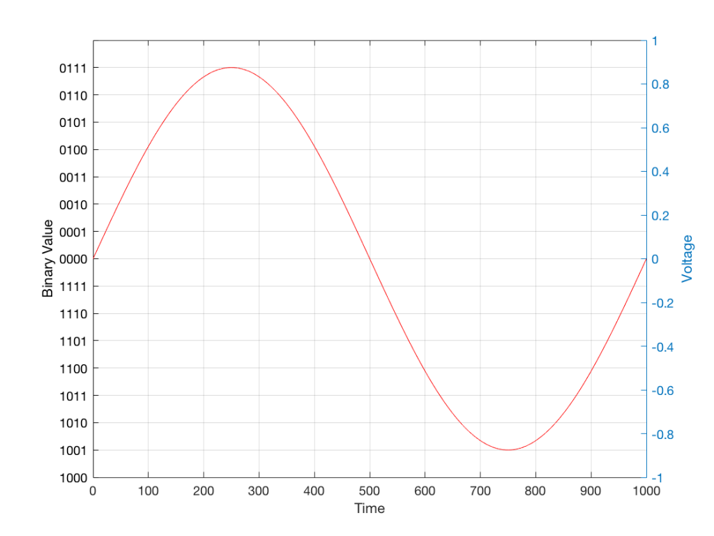
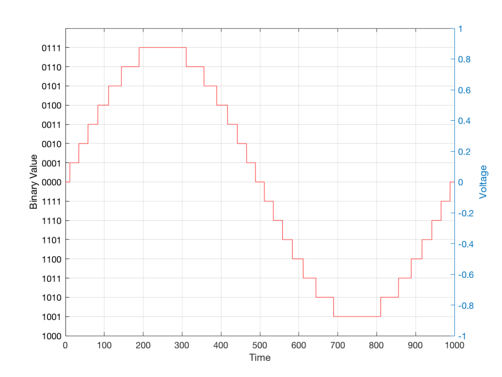
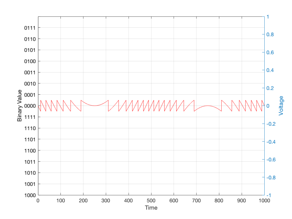
In some explanations of this problem, you may read that this error is called “quantisation noise”. However, this isn’t always correct. This is because if something is “noise” then is is random, and therefore impossible to predict. However, that’s not strictly the case for quantisation error. If you know the signal, and you know the quantisation values, then you’ll be able to predict exactly what the error will be. So, although that error might sound like noise, technically speaking, it’s not. This can easily be seen in Figures 1 through 3 which demonstrate that the quantisation error causes a periodic, predictable error (and therefore harmonic distortion), not a random error (and therefore noise).
Sidebar: The reason people call it quantisation noise is that, if the signal is complicated (unlike a sine wave) and high in level relative to the quantisation levels – say a recording of Britney Spears, for example – then the distortion that is generated sounds “random-ish”, which causes people to just to the conclusion that it’s noise.
Now, let’s talk about perception for a while… We humans are really good at detecting patterns – signals – in an otherwise noisy world. This is just as true with hearing as it is with vision. So, if you have a sound that exists in a truly random background noise, then you can focus on listening to the sound and ignore the noise. For example, if you (like me) are old enough to have used cassette tapes, then you can remember listening to songs with a high background noise (the “tape hiss”) – but it wasn’t too annoying because the hiss was independent of the music, and constant. However, if you, like me, have listened to Bob Marley’s live version of “No Woman No Cry” from the “Legend” album, then you, like me, would miss the the feedback in the PA system at that point in the song when the FoH engineer wasn’t paying enough attention… That noise (the howl of the feedback) is not noise – it’s a signal… Which makes it just as important as the song itself. (I could get into a long boring talk about John Cage at this point, but I’ll try to not get too distracted…)
The problem with the signal in Figure 2 is that the error (shown in Figure 3) is periodic – it’s a signal that demands attention. If the signal that I was sending into the quantisation system (in Figure 1) was a little more complicated than a sine wave – say a sine wave with an amplitude modulation – then the error would be easily “trackable” by anyone who was listening.
So, what we want to do is to quantise the signal (because we’re assuming that we can’t make a better “ruler”) but to make the error random – so it is changed from distortion to noise. We do this by adding noise to the signal before we quantise it. The result of this is that the error will be randomised, and will become independent of the original signal… So, instead of a modulating signal with modulated distortion, we get a modulated signal with constant noise – which is easier for us to ignore. (It has the added benefit of spreading the frequency content of the error over a wide frequency band, rather than being stuck on the harmonics of the original signal… but let’s not talk about that…)
For example…
Let’s take a look at an example of this from an equivalent world – digital photography.
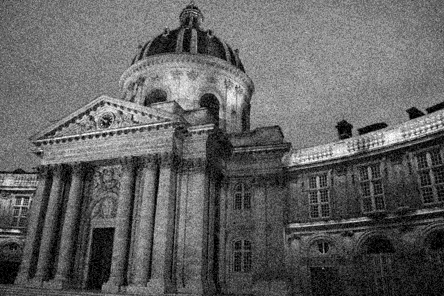
The photo in Figure 4 is a black and white photo – which actually means that it’s comprised of shades of gray ranging from black all the way to white. The photo has 272,640 individual pixels (because it’s 640 pixels wide and 426 pixels high). Each of those pixels is some shade of gray, but that shading does not have an infinite resolution. There are “only” 256 possible shades of gray available for each pixel.
So, each pixel has a number that can range from 0 (black) up to 255 (white).

If we were to zoom in to the top left corner of the photo and look at the values of the 64 pixels there (an 8×8 pixel square), you’d see that they are:
86 86 90 88 87 87 90 91
86 88 90 90 89 87 90 91
88 89 91 90 89 89 90 94
88 90 91 93 90 90 93 94
89 93 94 94 91 93 94 96
90 93 94 95 94 91 95 96
93 94 97 95 94 95 96 97
93 94 97 97 96 94 97 97
What if we were to reduce the available resolution so that there were fewer shades of gray between white and black? We can take the photo in Figure 1 and round the value in each pixel to the new value. For example, Figure 5 shows an example of the same photo reduced to only 4 levels of gray.

Now, if we look at those same pixels in the upper left corner, we’d see that their values are
102 102 102 102 102 102 102 102
102 102 102 102 102 102 102 102
102 102 102 102 102 102 102 102
102 102 102 102 102 102 102 102
102 102 102 102 102 102 102 102
102 102 102 102 102 102 102 102
102 102 102 102 102 102 102 102
102 102 102 102 102 102 102 102
They’ve all been quantised to the nearest available level, which is 102. (Our possible values are restricted to 0, 51, 102, 154, 205, and 255).
So, we can see that, by quantising the gray levels from 256 possible values down to only 6, we lose details in the photo. This should not be a surprise… That loss of detail means that, for example, the gentle transition from lighter to darker gray in the sky in the original is “flattened” to a light spot in a darker background, with a jagged edge at the transition between the two. Also, the details of the wall pillars between the windows are lost.
If we take our original photo and add noise to it – so were adding a random value to the value of each pixel in the original photo (I won’t talk about the range of those random values…) it will look like Figure 6. This photo has all 256 possible values of gray – the same as in Figure 1.

If we then quantise Figure 6 using our 6 possible values of gray, we get Figure 7. Notice that, although we do not have more grays than in Figure 5, we can see things like the gradual shading in the sky and some details in the walls between the tall windows.
That noise that we add to the original signal is called dither – because it is forcing the quantiser to be indecisive about which level to quantise to choose.
I should be clear here and say that dither does not eliminate quantisation error. The purpose of dither is to randomise the error, turning the quantisation error into noise instead of distortion. This makes it (among other things) independent of the signal that you’re listening to, so it’s easier for your brain to separate it from the music, and ignore it.
Addendum: Binary basics and SNR
We normally write down our numbers using a “base 10” notation. So, when I write down 9374 – I mean
9 x 1000 + 3 x 100 + 7 x 10 + 4 x 1
or
9 x 10³ + 3 x 10² + 7 x 101 + 4 x 100
We use base 10 notation – a system based on 10 digits (0 through 9) because we have 10 fingers.
If we only had 2 fingers, we would do things differently… We would only have 2 digits (0 and 1) and we would write down numbers like this:
11101
which would be the same as saying
1 x 16 + 1 x 8 + 1 x 4 + 0 x 2 + 1 x 1
or
1 x 24 + 1 x 23 + 1 x 22 + 0 x 21 + 1 x 20
The details of this are not important – but one small point is. If we’re using a base-10 system and we increase the number by one more digit – say, going from a 3-digit number to a 4-digit number, then we increase the possible number of values we can represent by a factor of 10. (in other words, there are 10 times as many possible values in the number XXXX than in XXX.)
If we’re using a base-2 system and we increase by one extra digit, we increase the number of possible values by a factor of 2. So XXXX has 2 times as many possible values as XXX.
Now, remember that the error that we generate when we quantise is no bigger than 1/2 of a quantisation step, regardless of the number of steps. So, if we double the number of steps (by adding an extra binary digit or bit to the value that we’re storing), then the signal can be twice as “far away” from the quantisation error.
This means that, by adding an extra bit to the stored value, we increase the potential signal-to-error ratio of our LPCM system by a factor of 2 – or 6.02 dB.
So, if we have a 16-bit LPCM signal, then a sine wave at the maximum level that it can be without clipping is about 6 dB/bit * 16 bits – 3 dB = 93 dB louder than the error. The reason we subtract the 3 dB from the value is that the error is +/- 0.5 of a quantisation step (normally called an “LSB” or “Least Significant Bit”).
Note as well that this calculation is just a rule of thumb. It is neither precise nor accurate, since the details of exactly what kind of error we have will have a minor effect on the actual number. However, it will be close enough.