#8 in a series of articles about wander and jitter

Ignoring a most of the details, converting an analogue audio signal into a digital one is much like filming a movie. The signal (a continuous change in voltage) is measured (or sampled) at a regular rate (the sampling rate), and those measurements are stored for future use. This is called Analogue-to-Digital Conversion.

In the future, you take those samples, and you convert them back to voltages at the same sampling rate (in the same way that you play a film at the same frame rate that you used to record it). This is called Digital-to-Analogue Conversion.

However, we’re not here to talk about conversion – we’re here to talk about jitter in the conversion process.

As we’ve already seen, jitter (and wander) is an error in the timing of a clock event. So, let’s look at this effect as part of the sampling process. To start: jitter in the analogue to digital conversion.

Jitter in the Analogue to Digital conversion

Let’s say that we want to convert an analogue sinusoidal wave into a PCM digital version.

Note that I’m going to skip a bunch of steps in the following explanation – concentrating only on the parts that are important for our discussion of jitter.

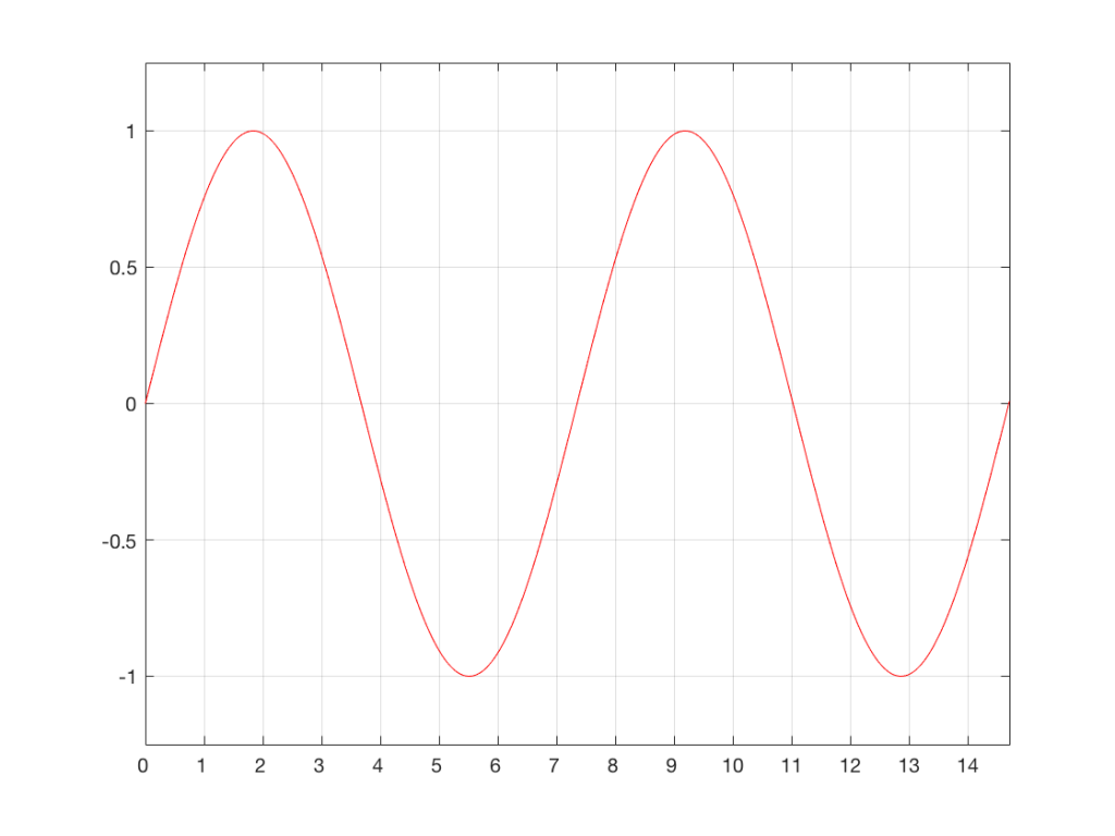
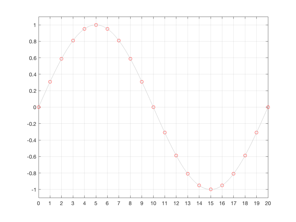
We start with a wave that has theoretically infinite resolution in amplitude and time, and we divide time into discrete moments, represented by the numbered vertical lines in the plot below.

Every time the clock “ticks” (in other words, on each of those vertical lines), we measure the voltage of the signal. These discrete measurements are represented in Figure 2 as the circles, sitting on the original waveform (in gray).

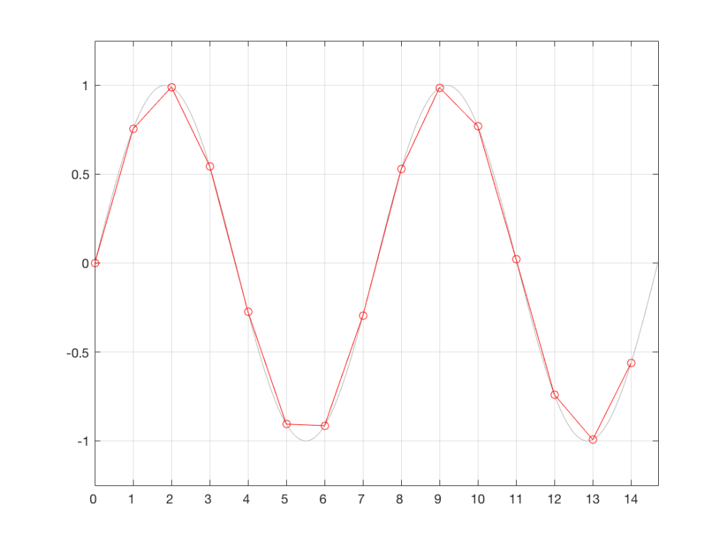
Part of this system relies on the accuracy of the clock that’s used to tell the sampling system when to do the measurements. In a perfect world, a system with a sampling rate of 44.1 kHz would make a measurement of the incoming analogue wave exactly every 1/44100th of a second. The time between samples would never vary.

This, of course, is impossible. The clock that ticks at the sampling rate will have some error in time – albeit a very, very small error.

Let’s heavily exaggerate this error so that we can see the resulting effect. Figure 3 shows the same original analogue sinusoidal waveform, sampled (measured) at incorrect times. In other words, sometimes the measurement (represented by the red circles) is made slightly too early (to the left of the gray vertical line – as is the case for Sample #9), sometimes, it’s made too late (to the right of the line – as in Sample #2).

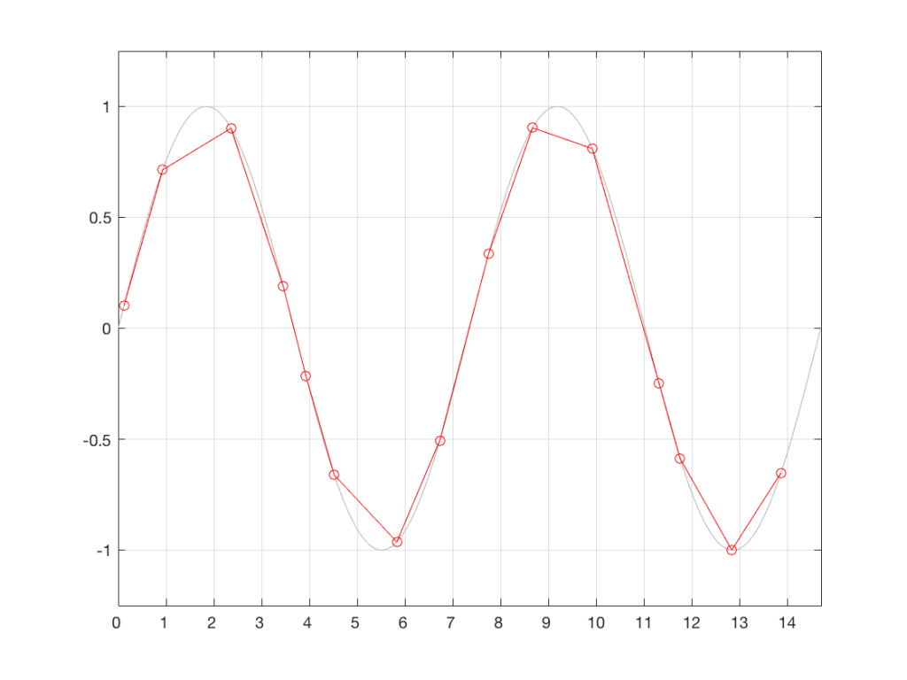
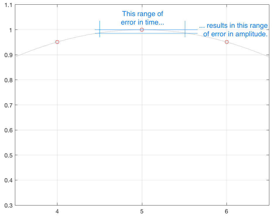
For example, look at the sample that should occur at clock tick #2. I’ve zoomed in to the plot so that this can be seen more clearly in Figure 4.

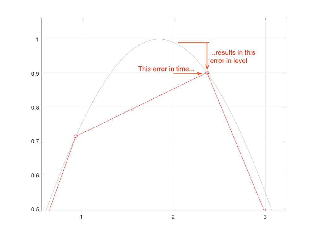
Notice that, because the measurement was made at the wrong time (in the case of sample #2, somewhat late), the result is an error in the measurement of the waveform’s amplitude. So, an error in time produces an error in level.

Let’s assume that the measurements we made in Figure 3 are stored and then replayed at exactly the correct times – what will the result be? This is shown in Figure 5. As you can see there, by comparing the measurements we made in Figure 3 to the original waveform, we have resulted in a distortion of the waveform.

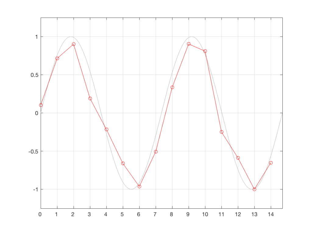
The time-based errors in the measurements in Figure 3 result (in this example) in a system that contains amplitude-based errors at the output. This results in some kind of distortion of the signal, as can be seen here.

As you can see in Figure 5, the result is a signal that is not a sine wave. Even after this digital signal has been low-pass filtered by the reconstruction filter in the Digital-to-Analogue Converter (the DAC), it will not be a clean sine wave. But let’s think about exactly what can go wrong here, more carefully.

For starters, an error that is ONLY caused by timing errors in the sampling process cannot produce levels that are outside the amplitude range of the original signal. In other words, if our original signal was 1 V Peak and symmetrical, then the sampled waveform will not exceed this. This is because the samples are all real measurements of the signal – merely performed at the incorrect times.

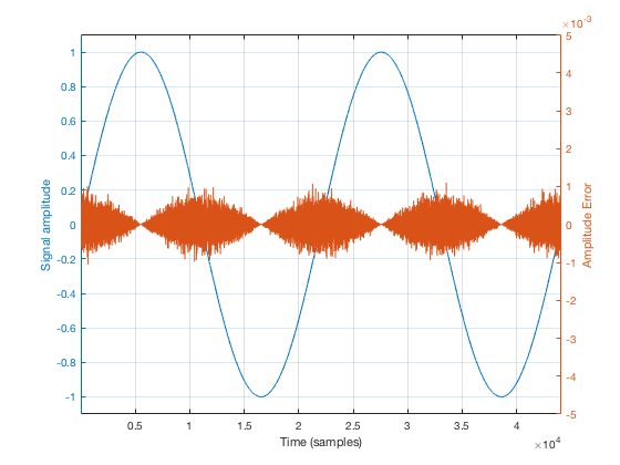
Secondly, if the amount of jitter is kept constant, then the amount of amplitude error will modulate (or vary) with the slope of the signal. This is illustrated in Figure 6, below.

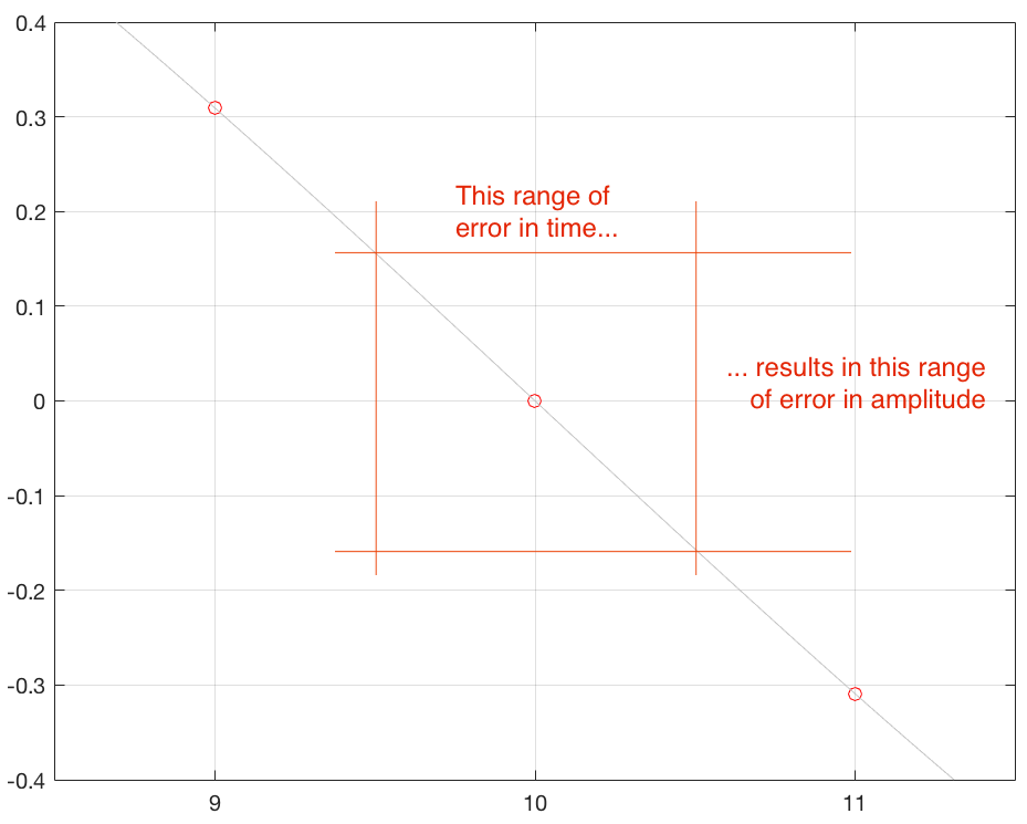
Another way to consider this is that, given a constant amount of jitter, the amplitude error (and therefore the distortion that is generated) modulates with the signal, is proportional to the slope of the signal. Since the maximum slope of the signal increases with amplitude and with frequency, then jitter artefacts will also increase as a result of an increase in the signal level or its frequency.

Thirdly, (and this one may be obvious): in an LPCM system, there are no jitter artefacts if there is no signal. If the input signal is constantly 0, then it doesn’t matter when you measure it… (Note that I said “in an LPCM system” in that sentence – if it’s a Delta-Sigma (1-bit) converter, then this is not true.)

There is more thing to consider  – although, given the level of jitter in real-life systems these days, this one is more of a thought experiment than anything else. Take a look back at Figure 3 – specifically, the samples that should have been taken at times 11 and 12. In a 44.1 kHz system, those two samples would have been samples 1/44100th of a second apart. However, as you can see there, the time between those two samples is less than 1/44100th of a second. If the sampling period is reduced, then the sampling rate must be higher than 44.1 kHz. This means that, ignoring everything else, the Nyquist frequency of the system is momentarily raised, allowing content above the intended Nyquist into the captured signal… However, as I said, this is merely an interesting thing to think about. Find something else to feed your free-floating anxiety that keeps you up at night – this issue is not worth a wink’s worth of lost sleep…

One extra thing to note here: If you look at Figure 3, you see a signal that has artefacts caused by jitter. Simply stated, this means that there are errors in the recorded signal. The way I’ve plotted this in Figure 3, those can be considered to be amplitude errors when played through a system without jitter. In other words, if you have a signal with jitter artefacts, you cannot remove them by using a system that has no jitter. the best you can do is to not add more jitter…

Addendum: This description of jitter artefacts as an amplitude distortion is only one way to look at the problem – using what is called the “Time-Domain Model”. Instead, you could use the “Frequency-Domain Model”, which I will not discuss here. If you’d like to dive into this further, Julian Dunn’s paper called “Jitter Theory” – Technical Note TN-23 from Audio Precision is the best place to start. This is a chapter in his book called “Measurement Techniques for Digital Audio”, published by Audio Precision. See this link for more info.