#8 in a series of articles about wander and jitter
In the previous post we looked at the effect of an incoming analogue signal that is sampled at the wrong times. In that description, I implied that the playback of the samples would happen at exactly the correct times. So, the jitter was entirely at the ADC (analogue-to-digital converter) and nowhere else.
In this posting, we’ll look at a very similar issue – jitter in the DAC (digital-to-analogue converter).
Jitter in the Digital to Analogue conversion
Let’s assume that we have a signal (in our case, a sinusoidal waveform, since that’s easy to plot) that was sampled by an ADC with no jitter. So, our original signal looks like Figure 1.
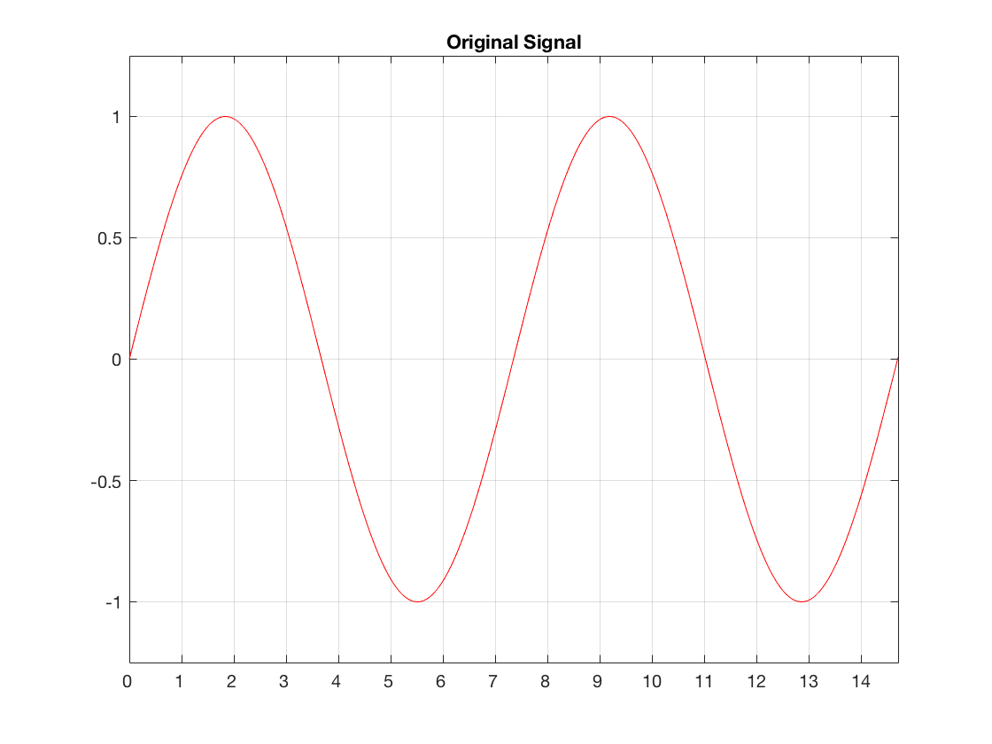
Fig 1. The original waveform. The x-axis shows time, divided into the sample times when we’re doing the measurements of the signal.
That signal is sampled by the ADC at exactly the correct times, since it has no jitter. The result of this is shown below in Figure 2.
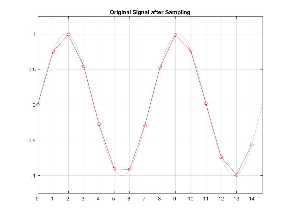
Fig 2. The original waveform (in gray) and the samples that are measured by the ADC.
When the time comes to play this signal, we send those samples to the DAC in the correct order and hope that it converts each of them to an analogue voltage at exactly the correct times. If the sampling rate of the system is 96 kHz, then we hope that the DAC converts a sample ever 1/96000th of a second, at exactly the right time each time.
That time that the DAC spits out the sample is dictated by a clock somewhere in the system. It might by an internal clock, or it might come from an external device, depending on your system and how it’s being used. However, if that clock is inaccurate for some reason, or if there is some kind of noise infecting the connection between the clock and the DAC, then the DAC can be triggered to convert a sample at the incorrect time. This is sampling jitter in the digital to analogue conversion process. I’ve tried to illustrate this in Figure 3.
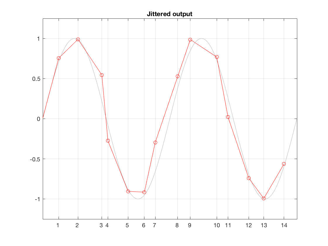
Fig 3. An illustration of jitter at the digital to analogue conversion process. Notice that the times between consecutive samples is not consistent.
It may not be immediately obvious, but the sample values in Figure 3 are identical to those in Figure 2. What I’ve done is to move them in time, so that you’re getting exactly the right level output at the wrong time each time. Of course, I have heavily exaggerated this plot to make it obvious that the times between consecutive samples are not equal. Some are much shorter than the sampling period (e.g. between samples 3 and 4) and some are much longer (e.g between samples 9 and 10).
Just like the case of ADC jitter, we can analyse this simply as an amplitude error. In other words, as a result of the timing errors, the red circles are not sitting directly on the original gray signal. And, just like we saw in the case of the ADC jitter, the amount of amplitude error is proportional to the slope of the signal.
Addendum: It’s important to remember that the descriptions and the plots that I’m showing here are to help show what jitter is – and those plots are high. I’m not showing what the final result will be. The actual jitter in a system is much, much lower than anything I’ve shown here. Also, I’ve completely omitted the effects of the anti-aliasing filter and the reconstruction filter – just to keep things simple.