#7 in a series of articles about wander and jitter
Back in a previous posting, we looked at this plot:
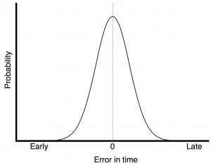
The plot in Figure 1 shows the probability of a timing error when you have random jitter. The highest probability is that the clock event will happen at the correct time, with no error. As the error increases (either earlier or later) the probability of that happening decreases – with a Gaussian distribution.
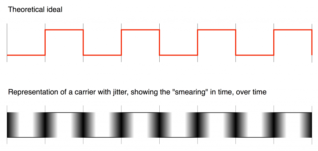
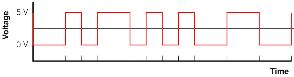
As we already saw, this means that (if the system had an infinite bandwidth, but random jitter) the incoming signal would look something like the bottom plot in Figure 2 when it should look like the top plot in the same Figure.
However, Figure 1 doesn’t really give us enough information. It tells us something about the timing error of a single event – but we need to know more.
Sidebar: Encoding, Transmitting, and Decoding a bi-phase mark
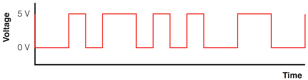
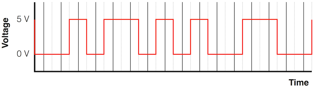
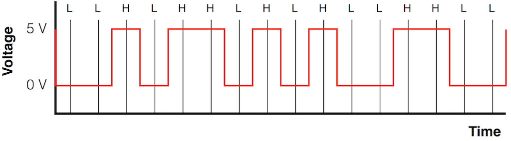
Let’s say that you wanted to transmit the sequence of bits 01011000 through a system that used the bi-phase mark protocol (like S-PDIF, for example). Let’s walk through this, step by step, using the following 7 diagrams.
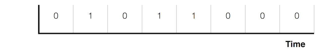
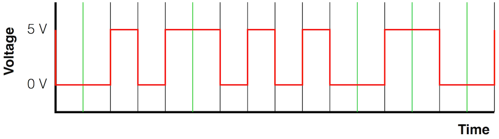
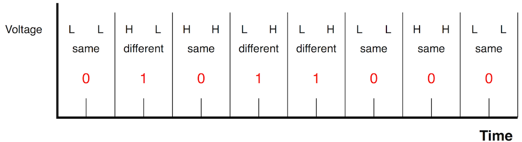
At this point, the receiver has two pieces of information:
- the binary string of values – 01011000
- a series of clock “ticks” that matches double the bit rate of the incoming signal
How do we get a data error?
The probability plot in Figure 1 shows the distribution of timing errors for a single clock event. What it does not show is how that relates to the consecutive events. Let’s look at that.
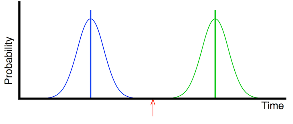
Let’s say that you have two consecutive clock events, represented in Figure 10, below, as the vertical Blue and Green lines. If you have jitter, then there is some probability that those events will be either early or late. If the jitter is random jitter, then the distribution of those probabilities are Gaussian and might look something like the pretty “bell curves” in Figure 10.
Basically, this means that the clock event that should happen at the time of the vertical blue line might happen anywhere in time that is covered by the blue bell curve. This is similarly true for the clock event marked with the green lines.
If we were to represent this as the actual pulse wave, it would look something like Figure 11, below.
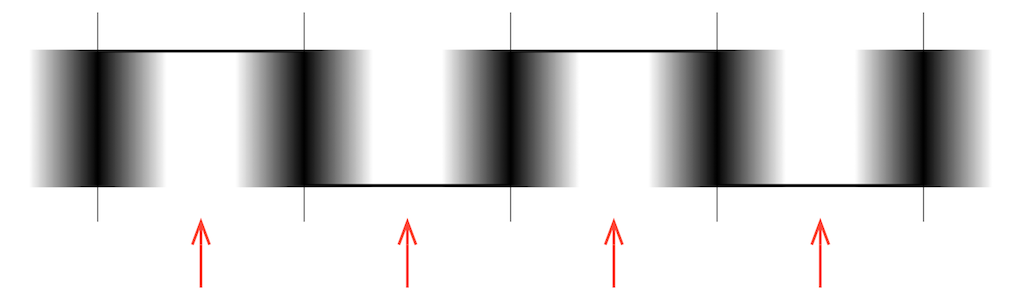
You will see some red arrows in both Figure 10 and Figure 11. These indicate the time between detected clock events, which the receiver decides is the “safe” time to detect whether the voltage of the carrier signal is “high” or “low”. As you can probably see in both of these plots, the signal at the moments indicated by the red arrows is obviously high or low – you won’t make a mistake if you look at the carrier signal at those times.
However, what if the noise level is higher, and therefore the jitter is worse?
In this case, the actual clock events don’t move in time – but their probability curves widen – meaning that the error can be earlier or later than it was before. This is shown in Figure 12, below.
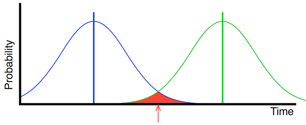
If you look directly above the red arrow in Figure 12, you will see that both the blue line and the green line are there… This means that there is some probability that the first clock event (the blue one) could come AFTER the second (the green one). That time reversal could happen any time in the range covered by the red area in the plot.
An artist’s representation of this in time is shown in Figure 13, below. Notice that there is no “safe” place to detect whether the carrier signal’s voltage is high or low.
If this happens, then the sequence that should be interpreted as 1-0 becomes 0-1 or vice versa. Remember that this is happening at the carrier signal’s cell rate – not the audio bit rate (which is one-half of the cell rate because there are two cells per bit) – so this will result in an error – but let’s take a look at what kind of error…
The table below shows a sequence of 3 binary values on the left. The next column shows the sequence of High and Low values that would represent that sequence, with two values in red – which we assume are reversed. The third column shows the resulting sequence. The right-most column shows the resulting binary sequence that would be decoded, including the error. If the binary sequence is different from the original, I display the result in red.
You will notice that some errors in the encoded signal do not result in an error in the decoded sequence. (HH and LL are reversed to be HH and LL.)
You will also notice that I’ve marked some results as “Invalid”. This happens in a case where the cells from two adjacent bits are the same. In this case, the decoder will recognise that an error has occurred.
[table]
Original, Encoded, Including error, Decoded
000, HH LL HH, HH LL HH, 000
,HH LL HH, HL HL HH, 110
, HH LL HH, HH LL HH, 000
,HH LL HH, HH LH LH, 011
, HH LL HH, HH LL HH, 000
001, HH LL HL, HH LL HL, 001
, HH LL HL, HL HL HL, 111
, HH LL HL, HH LL HL, 001
, HH LL HL, HH LH LL, 010
, HH LL HL, HH LL LH, Invalid
010, HH LH LL, HH LH LL, 010
, HH LH LL, HL HH LL, 100
, HH LH LL, HH HL LL, Invalid
, HH LH LL, HH LL HH, 000
, HH LH LL, HH LH LL, 010
100, HL HH LL, LH HH LL, Invalid
, HL HH LL, HH LH LL, 010
, HL HH LL, HL HH LL, 100
, HL HH LL, HL HL HL, 111
, HL HH LL, HL HH LL, 100
011, HH LH LH, HH LH LH, 011
, HH LH LH, HL HH LH, 101
, HH LH LH, HH HL LH, Invalid
, HH LH LH, HH LL HH, 000
, HH LH LH, HH LH HL, Invalid
110, HL HL HH, LH HL HH, Invalid
, HL HL HH, HH LL HH, 000
, HL HL HH, HL LH HH, Invalid
, HL HL HH, HL HH LH, 101
, HL HL HH, HL HL HH, 110
111, HL HL HL, LH HL HL, Invalid
, HL HL HL, HH LL HL, 001
, HL HL HL, HL LH HL, Invalid
, HL HL HL, HL HH LL, 100
, HL HL HL, HL HL LH, Invalid
[/table]
How often might we get an error?
As you can see in the table above, for the 5 possible errors in the encoded stream, the binary sequence can have either 2, 3, or 4 errors (or invalid cases), depending on the sequence of the original signal.
If we take a carrier wave that has random jitter, then its distribution is Gaussian. If it’s truly Gaussian, then the worst-case peak-to-peak error that’s possible is infinity. Of course, if you measure the peak-to-peak error of the times of clock events in a carrier wave (a range of time), it will not be infinity – it will be a finite value.
We can also measure the RMS error of the times of clock events in a carrier wave, which will be a smaller range of time than the peak-to-peak value.
We can then calculate the ratio of the peak-to-peak value to the RMS value. (This is similar to calculating the crest factor – but we use the peak-to-peak value instead of the peak value.) This will give you and indication of the width of the “bell curve”. The closer the peak-to-peak value is to the RMS value (the lower the ratio) the wider the curve and the more likely it is that we will get bit errors.
The value of the peak-to-peak error divided by the RMS error can be used to calculate the probability of getting a data error, as follows:
[table]
Peak-to-Peak error / RMS error, Bit Error Rate
12.7, 1 x 10⁻⁹
13.4, 1 x 10⁻¹⁰
14.1, 1 x 10-11
14.7, 1 x 10-12
15.3, 1 x 10-13
[/table]
The Bit Error Rate is a prediction of how many errors per bit we’ll get in the carrier signal. (It is important to remember that this table shows a probability – not a guarantee. Also, remember that it shows the probability of Data Errors in the carrier stream – not the audio signal.)
So, for example, if we have an audio signal with a sampling rate of 192 kHz, then we have 192,000 kHz * 32 bits per audio sample * 2 channels * 2 cells per bit = 24,576,000 cells per second in the S-PDIF signal. If we have a BER (Bit Error Rate) of 1 x 10⁻⁹ (for example) then we will get (on average) a cell reversal approximately every 41 seconds (because, at a cell rate of 24,576,000 cells per second, it will take about 41 seconds to get to 109 cells). Examples of other results (for 192 kHz and 44.1 kHz) are shown in the tables below.
[table]
Bit Error Rate, Time per error (192 kHz)
1 x 10⁻⁹, 41 seconds
1 x 10⁻¹⁰, 6.78 minutes
1 x 10-11, 67.8 minutes
1 x 10-12, 11.3 hours
1 x 10-13, 4.7 days
[/table]
[table]
Bit Error Rate, Time per error (44.1 kHz)
1 x 10⁻⁹, 2.95 minutes
1 x 10⁻¹⁰, 29.53 minutes
1 x 10-11, 4.92 hours
1 x 10-12, 2.05 days
1 x 10-13, 20.5 days
[/table]
You may have raised an eyebrow with the equation above – when I assumed that there are 32 bits per sample. I have done this because, even when you have a 16-bit audio signal, that information is packed into a 32-bit long “word” inside an S-PDIF signal. This is leaving out some details, but it’s true enough for the purposes of this discussion.
Finally, it is VERY important to remember that many digital audio transmission systems include error correction. So, just because you get a data error in the carrier stream does not mean that you will get a bit error in the audio signal.