In Part 2, I showed the raw magnitude response results of three pairs of headphones measured on three different systems, each done 5 times. However, when you plot magnitude responses on a scale with 80 dB like I did there, it’s difficult to see what’s going on.
Differences in measurements relative to average
One way to get around this issue is to ignore the raw measurement and look at the differences between them, which is what we’ll do here. This allows us to “zoom in” on the variations in the measurements, at the cost of knowing what the general overall responses are.
Figure 1 in Part 2 showed the 5 x 3 sets of raw magnitude responses of the open headphones. I then take each set of 5 measurements (remember that these 5 measurements were done by removing the headphones and re-setting them each time on the measurement rig) and find their average response. Then I plot the difference between each of the 5 measurements and that average, and this is done for each of the three measurement systems, as shown below in Figure 1.
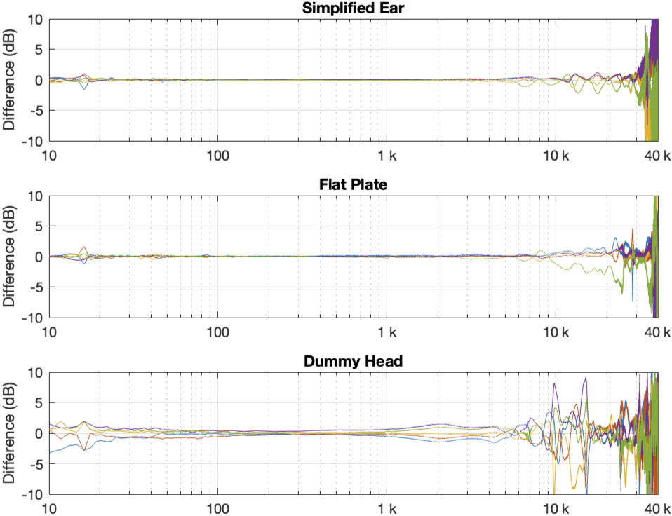
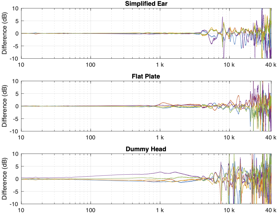
Some of the things that were intuitively visible in the plots in Part 2 are now obvious:
- There is a huge change in the measured magnitude response in the high frequency bands, even when the pair of headphones and the measurement rig are the same. This is the result of small changes in the physical position of the headphones on the rig, as well as changes in the clamping force (modified by moving the headband extension). I intentionally made both of these “errors” to show the problem. Notice that the differences here are greater than ±10 dB, which is a LOT.
- Overall, the differences between the measurements on the dummy head are bigger and have a lower frequency range than for the other two systems. This is mostly due to two things:
- because the dummy head has pinnae (ears), very small changes in position result in big changes in response
- it is easier to have small leaks around the ear cushions on a dummy head than with a flat surrounding of a metal plate or an artificial ear. This is the reason for the low-frequency differences with the closed headphones. Leaks have no effect on open headphone designs, since they are always leaking out through the diaphragm itself.
The differences that you can see here are the reason that, when we’re measuring headphones, we never measure just once. We always do a minimum of 5 measurements and look at the average of the set. This is standard practice, both for headphone developers and experienced reviewers like this one, for example.
In addition to this averaging, it’s also smart to do some kind of smoothing (which I have not done here…) to avoid being distracted by sharp changes in the response. Sharp peaks and dips can be a problem, particularly when you look at the phase response, the group delay, or looking for ringing in the time domain. However, it’s important to remember that the peaks and dips that you see in the measurements above might not actually be there when you put the headphones on your head. For example, if the variations are caused by standing waves inside the headphones due to the fact that the measurement system itself is made of reflective plastic or metal (but remember that you aren’t…) then the measurement is correct, but it doesn’t reflect (ha ha…) reality…
One additional thing to remember with these plots is that something that looks like a peak in the curve MIGHT be a peak, but it might also be a dip in the average curve because we’re only looking at the differences in the responses.
System differences
Instead of looking at the differences between each individual measurement and the average of the measurement set, we can also look at the differences between what each measurement system is telling us for each headphone type. For example, if I take one measurement of a pair of headphones on each system, and pretend that one of them is “correct”, then I can find the difference between the measurements from the other two systems and that “reference”.
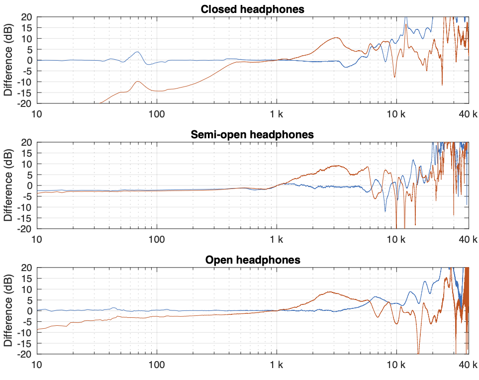
In Figure 4, I’m pretending that the flat plate is the “correct” system, and then I’m plotting the difference between the dummy head measurement (in red) and the artificial ear measurement (in blue) relative to it.
Again, it’s important to remember with these plots is that something that looks like a peak in the curve might actually be a dip in the “reference” curve. (The bump in the red lines around 2 – 3 kHz is an example of this…)
Of course, you could say “but you just said that we shouldn’t look at a single measurement”… which is correct. If we use the averages of all 5 measurements for each set and do the same plot, the result is Figure 5.
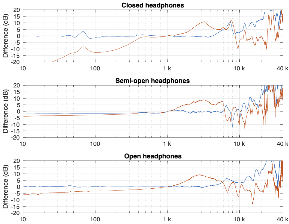
You can see there that, by using the averaged responses instead of individual measurements, the really sharp peaks and dips disappear, since they smooth each other out.
Comparing headphone types
Things get even more complicated if you try to compare the headphones to each other using the measurement systems. Figure 6, below, shows the averages of the five measurements of each pair of headphones on each measurement system, plotted together on the same graphs (normalised to the levels at 1 kHz), one for each measurement system.
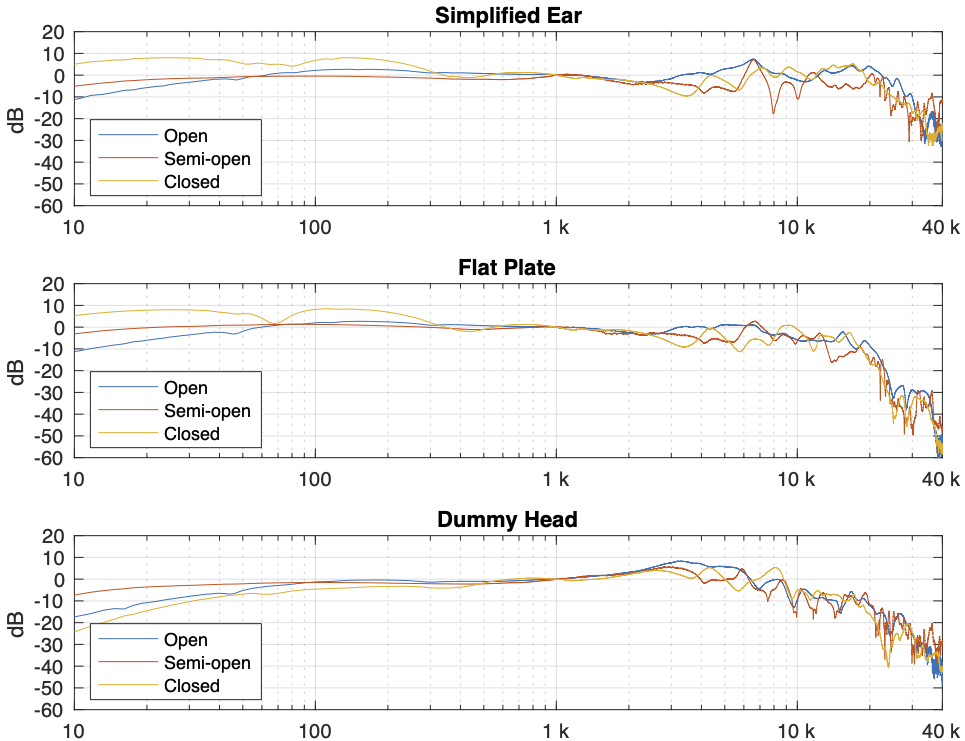
This is actually a really important figure, since it shows that the same headphones measured the same way on different systems tell you very different things. For example, if you use the “simplified ear” or the “flat plate” system, you’ll believe that the closed headphones (the yellow line) is about 10 – 15 dB higher than the open headphones (the blue line) in the low frequency region. However, if you use the “dummy head” system, you’ll believe that the closed headphones (the yellow line) is about 5 – 10 dB lower than the open headphones (the blue line) in the low frequency region.
Which one is correct? They all are, even though they tell you different things. After all, it’s just data… The reason this happens is that one measurement system cannot be used to directly compare two different types of headphones because their acoustic impedances are different. With experience, you can learn to interpret the data you’re shown to get some idea of what’s going on. However, “experience” in that sentence means “years of correlating how the headphones sound with how the plots look with the measurement system(s) you use”. If you aren’t familiar with the measurement system and how it filters the measurement, then you won’t be able to interpret the data you get from it.
That said, you MIGHT be able to use one system to compare two different pairs of open headphones or two different pairs of closed headphones, but you can’t directly compare measurements of different headphone types (e.g. open and closed) reliably.
This also means that, if you subscribe to two different headphone magazines both of which use measurements as part of their reviews, and one of them uses a flat plate system while the other uses a dummy head, the same pairs of headphones might get opposite reviews in the two magazines…
Which review can you trust? Both of them – and neither of them.
Conclusions
Looking at these plots, you could come to the conclusion that you can’t trust anything, because no two measurements tell you the same things about the same devices. This is the incorrect conclusion to draw. These measurement systems are tools that we use to tell us something about the headphones on which we’re working. And people who use these tools daily know how to interpret the data they see from them. If something looks weird, they either expected it to look weird, or they run the measurement on another system to get a different view.
The danger comes when you make one measurement on one device and hold that up as The Truth. A result that you get from any one of these systems is not The Truth, but it is A Truth – you just need more information. If you’re only shown one measurement (or even an average of measurements) that was done on only one measurement system, then you should raise at least one eyebrow, and ask some questions about how that choice of system affects the plots that you see.
In many ways, it’s like looking at a recipe in a cookbook. You might be able to determine whether you might like or probably hate a dish by reading its description of ingredients and how to prepare it. But you cannot know how it’ll taste until you make it and put it in your mouth. And, if you cook like I do, it’ll be just a little different next time. It’s cooking – not a chemistry experiment. If you use headphones like I do, it’ll also be a little different next time because some days, I don’t wear my glasses, or I position the head band a little differently, so the leak around the ear cushion or the clamping force is a little different.