One of my jobs at Bang & Olufsen is to do the final measurements on each bespoke Beogram 4000c turntable before it’s sent to the customer. Those measurements include checking the end-to-end magnitude response, playing from a vinyl record with a sine sweep on it (one per channel), recording that from the turntable’s line-level output, and analysing it to make sure that it’s as expected. Part of that analysis is to very that the magnitude responses of the left and right channel outputs are the same (or, same enough… it’s analogue, a world where nothing is perfect…)
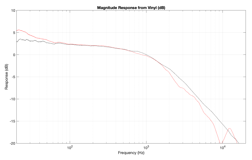
Today, I was surprised to see this result on a turntable that was being inspected part-way through its restoration process :
Taken at face value, this should have resulted in a rejection – or at least some very serious questions. This is a terrible result, with unacceptable differences in output level between the two channels. When I looked at the raw measurements, I could easily see that the left channel was behaving – it was the right channel that was all over the place.
The black curve looks very much like what I would expect to see. This is the result of playing a track that is a sine sweep from 20 Hz to 20 kHz, where the signal below 1 kHz follows the RIAA curve, whereas the signal above 1 kHz does not. This is why, after it’s been filtered using a RIAA preamp, the low frequency portion has a flat response, but the upper frequency band rolls off (following the RIAA curve).
Notice that the right channel (the red curve) is a mess…
A quick inspection revealed what might have been the problem: a small ball of fluff collected around the stylus. (This was a pickup that was being used to verify that the turntable was behaving through the restoration – not the one intended for the final customer – and so had been used multiple times on multiple turntables.)
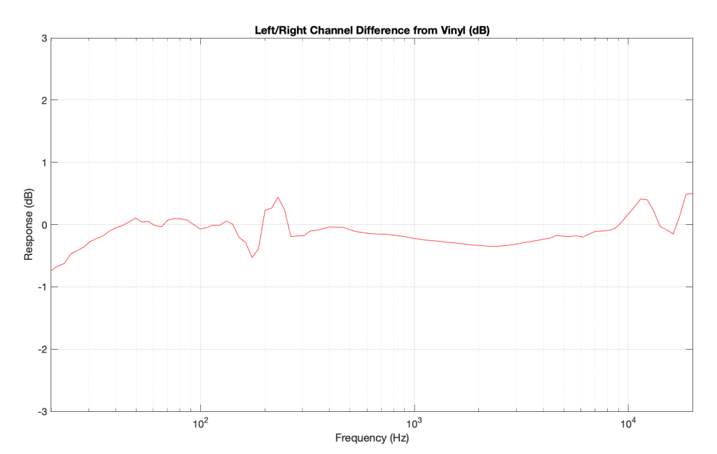
So, we used a stylus brush to clean off the fluff and ran the measurement again. The result immediately afterwards looked like this:
which is more like it! A left-right channel difference of something like ± 0.5 dB is perfectly acceptable.
The moral of the story: keep your pickup clean. But do it carefully! That cantilever is not difficult to snap.
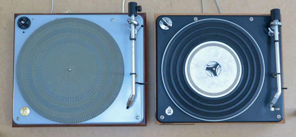
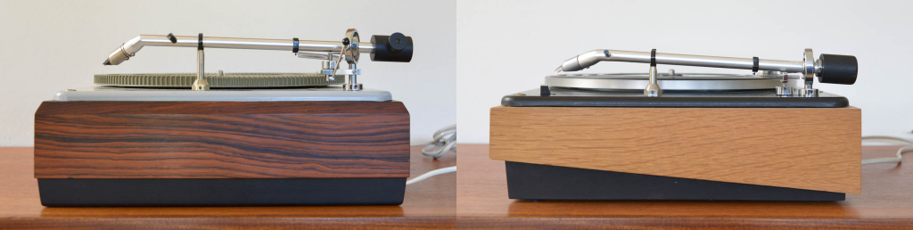
On the left: a “Stereopladespiller” (Stereo Gramophone) Type 42 VF. On the right, a Beogram 1000 V Type 5203 Series 33, modified with a built-in RIAA preamp (making it a Beogram 1000 VF)
Some history today – without much tech-talk. I just finished restoring my 42VF and I thought I’d spend an hour or two taking some photos next to my BG1000.
According to the beoworld.org website, the Stereopladespiller was in production from 1960 to 1976. Although Bang & Olufsen made many gramophones before 1960, they were all monophonic, for 1-channel audio. This one was originally made to support the 2-channel “SP1 / SP2” pickup developed by Erik Rørbæk Madsen after having heard 2-channel stereo on a visit to the USA in the mid-1950s (and returned to Denmark with a test record).
Sidebar: The “V” means that the players are powered from the AC mains voltage (220 V AC, 50 Hz here in Denmark). The “F” stands for “Forforstærker” or “Preamplifier”, meaning that it has a built-in RIAA preamp with a line-level output.
Internally, the SP1 and SP2 are identical. The only difference is the mounting bracket to accommodate the B&O “ST-” series tonearms and standard tonearms.
Name, Pivot – Platter Centre, Pivot – Stylus, Pickup
ST/M,190 mm, 205 mm, SP2
ST/L, 209.5 mm, 223.5 mm, SP2
ST/P, 310 mm, 320 mm, SP2
ST/A, 209.5 mm, 223.5 mm, SP1
[/table]
(I’ll do another, more detailed posting about the tonearms at a later date…)
Again, according to the beoworld.org website, the Beogram 1000 was in production from 1965 to 1973. (The overlap and the later EoP date of the former makes me a little suspicious. If I get better information, I’ll update this posting.)
The tonearm seen here on the Stereopladespiller is the ST/L model with a Type PL tonearm lifter.
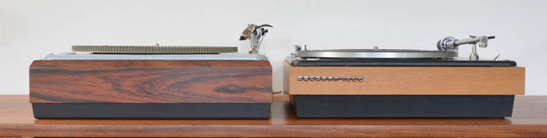
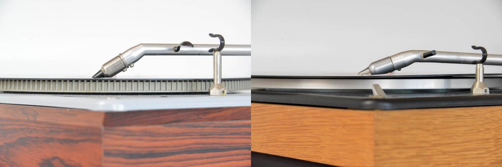
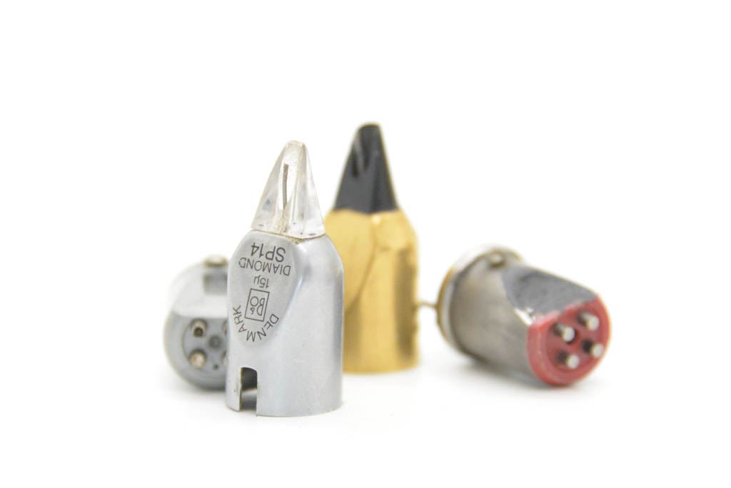
Looking not-very-carefully at the photos below, you can see that the two tonearms have a significant difference – the angle of the pickup relative to the surface of the vinyl. The ST/L has a 25º angle whereas the tonearm on the Beogram 1000 has a 15º angle. This means that the two pickups are mutually incompatible. The pickup shown on the Beogram 1000 is an SP14.
This, in turn, means that the vertical pivot points for the two tonearms are different, as can be seen below.
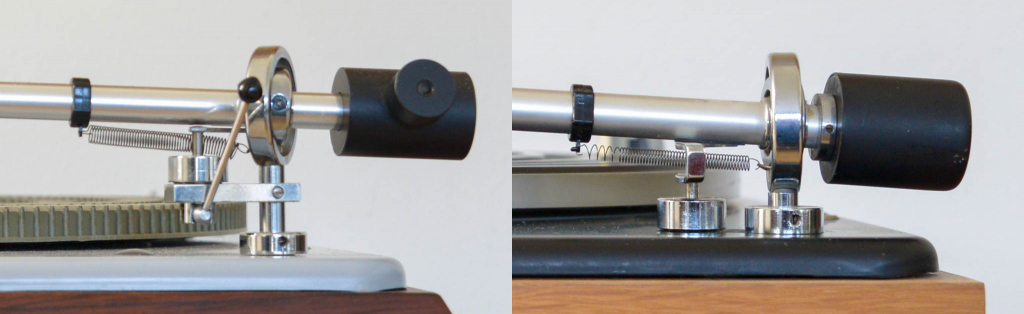
The heights of both tonearms at the pivot are adjustable by moving a collar around the post and fixing its position with a small set screw. A nut under the top plate (inside the turntable) locks it in position.
The position of the counterbalance on the older tonearm can be adjusted with the large setscrew seen in the photo above. The tonearm on the Beogram 1000 gently “locks” into the correct position using a small spring-loaded ball that sets into a hole at the end of the tonearm tube, and so it’s not designed to have the same adjustability.
Both tonearms use a spring attached to a plastic collar with an adjustable position for fine-tuning the tracking force. At the end of this posting, you can see that I’ve measured its accuracy.
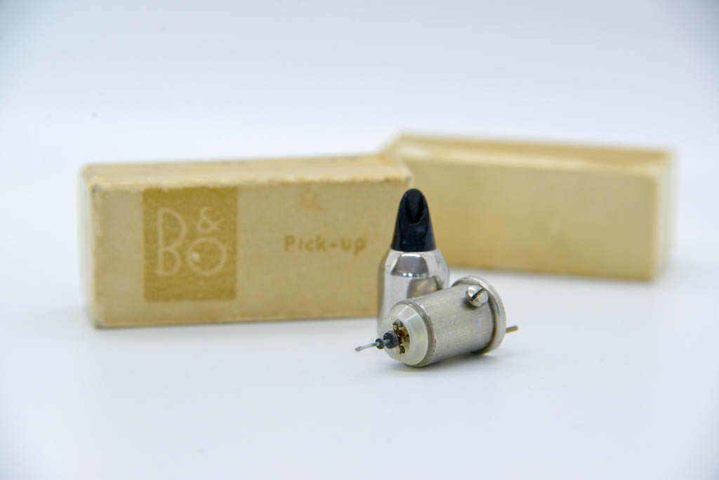
The Micro Moving Cross (MMC) principle of the SP1/2 pickup can easily be seen in the photo above (a New-Old-Stock pickup that I stumbled across at a flea market). For more information about the MMC design, see this posting. In later versions of the pickup, such as the SP14, seen below, the stylus and MMC assembly were attached to the external housing instead.
A couple of later SP-series pickups in considerably worse shape. These are also flea-market finds, but neither of them is behaving very well due to bent cantilevers.
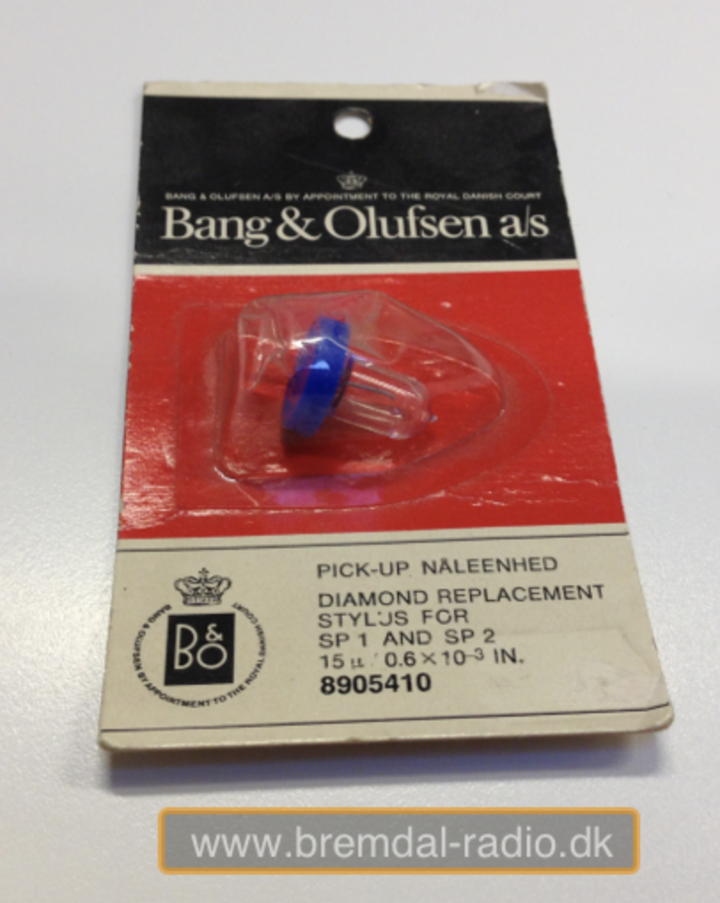
This construction made it easier to replace the stylus, although it was also possible to do so with the SP1-2 using a replacement such as the one shown below.
A replacement stylus for the SP1/2 shown on the bremdal-radio.dk website.
Just to satisfy my own curiosity, I measured the tracking force at the stylus with a number of different adjustments on the collar. The results are shown below.
Tracking force on the Stereopladespiller with the collar aligned to each side of the gradations on the tonearm. Right-click on the photo and open it in a new window or tab to zoom in for more details.Tracking force on the Beogram 1000 with the collar aligned to each side of the gradations on the tonearm. Right-click on the photo and open it in a new window or tab to zoom in for more details.
As you can see there, the accuracy is reasonably good. This is not really surprising, since the tracking force is applied by a spring. So, as long as the spring constant hasn’t changed over the years, which it shouldn’t have unless it got stretched for some reason (say, when I was rebuilding the pivot on the tonearm, for example…) it should behave as it always did.
There’s one last thing that I alluded to in a previous part of this series that now needs discussing before I wrap up the topic. Up to now, we’ve looked at how a filter behaves, both in time and magnitude vs. frequency. What we haven’t really dealt with is the question “why are you using a filter in the first place?”
Originally, equalisers were called that because they were used to equalise the high frequency levels that were lost on long-distance telephone transmissions. The kilometres of wire acted as a low-pass filter, and so a circuit had to be used to make the levels of the frequency bands equal again.
Nowadays we use filters and equalisers for all sorts of things – you can use them to add bass or treble because you like it. A loudspeaker developer can use them to correct linear response problems caused by the construction or visual design of the device. They can be used to compensate for the acoustical behaviour of a listening room. Or they can be used to compensate for things like hearing loss. These are just a few examples, but you’ll notice that three of the four of them are used as compensation – just like the original telephone equalisers.
Let’s focus on this application. You have an issue, and you want to fix it with a filter.
IF the problem that you’re trying to fix has a minimum phase characteristic, then a minimum phase filter (implemented either as an analogue circuit or in a DSP) can be used to “fix” the problem not only in the frequency domain – but also in the time domain. IF, however, you use a linear phase filter to fix a minimum phase problem, you might be able to take care of things on a magnitude vs. frequency analysis, but you will NOT fix the problem in the time domain.
This is why you need to know the time-domain behaviour of the problem to choose the correct filter to fix it.
For example, if you’re building a room compensation algorithm, you probably start by doing a measurement of the loudspeaker in a “reference” room / location / environment. This is your target.
You then take the loudspeaker to a different room and measure it again, and you can see the difference between the two.
In order to “undo” this difference with a filter (assuming that this is possible) one strategy is to start by analysing the difference in the two measurements by decomposing it into minimum phase and non-minimum phase components. You can then choose different filters for different tasks. A minimum phase filter can be used to compensate a resonance at a single frequency caused by a room mode. However, the cancellation at a frequency caused by a reflection is not minimum phase, so you can’t just use a filter to boost at that frequency. An octave-smoothed or 1/3-octave smoothed measurement done with pink noise might look like you fixed the problem – but you’ve probably screwed up the time domain.
Another, less intuitive example is when you’re building a loudspeaker, and you want to use a filter to fix a resonance that you can hear. It’s quite possible that the resonance (ringing in the time domain) is actually associated with a dip in the magnitude response (as we saw earlier). This means that, although intuition says “I can hear the resonant frequency sticking out, so I’ll put a dip there with a filter” – in order to correct it properly, you might need to boost it instead. The reason you can hear it is that it’s ringing in the time domain – not because it’s louder. So, a dip makes the problem less audible, but actually worse. In this case, you’re actually just attenuating the symptom, not fixing the problem – like taking an Asprin because you have a broken leg. Your leg is still broken, you just can’t feel it.
In order to explain the significance of the following story, some prequels are required.
Prequel #1: I’m one of those people who enjoys an addiction to collecting what other people call “junk” – things you find in flea markets, estate sales, and the like. Normally I only come home with old fountain pens that need to be restored, however, occasionally, I stumble across other things.
Prequel #2:Many people have vinyl records lying around, but not many people know how they’re made. The LP that you put on your turntable was pressed from a glob of molten polyvinyl-chloride (PVC), pressed between two circular metal plates called “stampers” that had ridges in them instead of grooves. Easy of those stampers was made by depositing layers of (probably) nickel on another plate called a “metal mother” which is essentially a metal version of your LP. That metal mother was made by putting layers on a “metal master” (also with ridges instead of grooves) which was probably a lamination of tin, silver, and nickel that was deposited in layers on an acetate lacquer disc, which is the original, cut on a lathe. (Yes, there are variations on this process, I know…) The thing to remember in this process is
there are three “playable” versions of the disc in this manufacturing process: your LP, the metal mother, and the original acetate that was cut on the lathe
there are two other non-playable versions that are the mirror images of the disc: the metal master and the stamper(s).
(If you’d like to watch this process, check out this video.)
Prequel #3: One of my recurring tasks in my day-job at Bang & Olufsen is to do the final measurements and approvals for the Beogram 4000c turntables. These are individually restored by hand. It’s not a production-line – it really is a restoration process. Each turntable has different issues that need to be addressed and fixed. The measurements that I do include:
verification of the gain and response of the two channels in the newly-built RIAA preamplifier (this is done electrically, by connecting the output of my sound card into the input of the RIAA instead of using a signal from the pickup)
checking the sensitivity and response of the two channels from vinyl to output
checking the wow and flutter of the drive mechanism
checking the channel crosstalk as well as the rumble
The last three of these are done by playing specific test tracks off an LP with signals on it, specifically designed for this purpose. There are sine wave sweeps, sine waves at different signal levels, a long-term sine wave at a high-ish frequency (for W&F measurements), and tracks with silence. (In addition, each turntable is actually tested twice for Wow and Flutter, since I test the platter and bearing before it’s assembled in the turntable itself…)
Prequel #4: Once-upon-a-time, Bang & Olufsen made their own pickup cartridges (actually, it goes back to steel needles). Initially the SP series, and then the MMC series of cartridges. Those were made in the same building that I work in every day – about 50 m from where I’m sitting right now. B&O doesn’t make the cartridges any more – but back when they did, each one was tested using a special LP with those same test tracks that I mentioned above. In fact, the album that they used once-upon-a-time is the same album that I use today for testing the Beogram 4000c. The analysis equipment has changed (I wrote my own Matlab code to do this rather than to dust off the old B&K measurement gear and the B&O Wow and Flutter meter…)
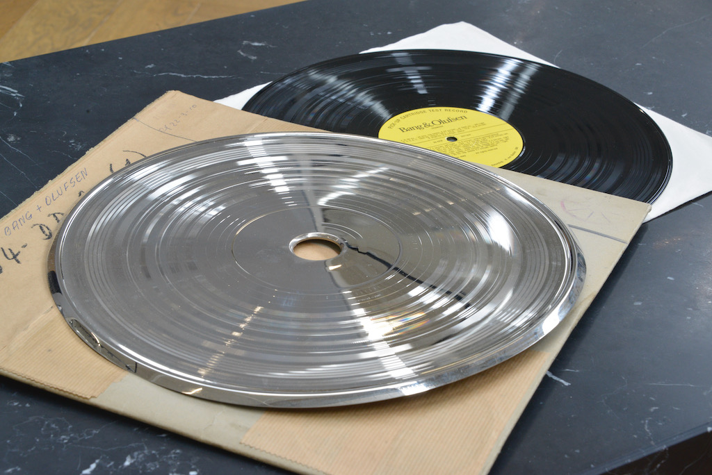
If you’ve read those four pieces of information, you’ll understand why I was recently excited to stumble across a stamper of the Bang & Olufsen test LP, with a date on the sleeve reading 21 March, 1974. It’s funny that, although the sleeve only says that it’s a Bang & Olufsen disc, I recognise it because of the pattern in the grooves (which should give you an indication of how many times I’ve tested the turntables) – even if they’re the mirror image of the vinyl disc.
Below, you can see my latest treasure, pictured with an example of the B&O test disc that I use. It hasn’t “come home” – but at least it’s moved in next-door.
P.S. Since a couple of people have already asked, the short answer is “no”. The long answers are:
No, the test disc is no longer available – it never was outside of the B&O production area. However, if you can find a copy of the Brüel and Kjær QR 2010 disc, it’s exactly the same. I suspect that the two companies got together to produce the test disc in the 70s. However, there were also some publicly-available discs by B&O that included some test tones. These weren’t as comprehensive as the “real” test discs like the ones accompanying the DIN standards, or the ones from CBS and JVC.
No, the metal master is no longer in good enough shape to use to make a new set of metal mothers and stampers. Too bad… :-(
P.P.S. If you’re interested in the details of how the tests are done on the Beogram 4000c turntables, I’ve explained it in the Technical Sound Guide, which can be downloaded using the link at the bottom of this page. That document also has a comprehensive reading list if you’re REALLY interested or REALLY having trouble sleeping.
As I’ve stated a couple of times through this series, my reason for writing this stuff was not to prove that high res audio is better or worse than normal res audio (whatever that is…). My reason was to highlight some of the advantages and disadvantages associated with LPCM audio at different bit depths and sampling rates. Just as a bullet-point summary of things-to-remember/consider (with some loose grouping):
“High resolution audio” could mean
“more than 16 bits per sample” or
“a sampling rate higher than 44.1 kHz” or
both.
These two dimensions of the specifications have different implications on the signal
Just because you have more bits per sample doesn’t mean that you are actually getting more resolution. There are examples out there where a “24-bit recording” is just a 16-bit recording with 8 zeros stuck on the end.
Just because you have a higher sampling rate doesn’t mean that you are actually getting a recording that was done at that sampling rate. There are examples out there where, if you do a spectral analysis of a “high-res” recording, you’ll see the cutoff filter of the original 44.1 kHz recording.
Just because you have a recording done at a higher sampling rate doesn’t mean that the extra information you get is actually useful.
If your processing distorts the signal for some reason, it’s better to have a higher sampling rate to keep the aliased distortion artefacts as far away from the audio signal as possible.
If you are a lazy DSP engineer who thinks that filters give you the expected magnitude response, no matter what the centre frequency, you’d better have a higher sampling rate. (Or you could just stop being lazy and compensate.)
If you need a lower noise floor for the same audio bandwidth, it’s more efficient to add bits than to increase the sampling rate.
If you have a volume control after the conversion to analogue, then 93 dB of dynamic range (16 bits, TPDF dithered) might be enough – especially if you listen to music with a limited dynamic range. However, if your volume control is in the digital domain, and you have a speaker that can play loudly, then you’ll probably want more dynamic range, and therefore more bits per sample hitting the DAC.
Like I said, I’m not here to tell you that one thing is better or worse than another thing.
As I said, my intention in writing all of this is to help you to never fall into the trap of assuming that “high resolution audio” is better than “normal resolution audio” in all respects.
More is not necessarily better, sometimes, it’s not even more. Don’t fall victim to misleading advertising.
This series has flipped back and forth between talking about high resolution audio files & sources and the processing that happens in the equipment when you play it. For this posting, we’re going to deal exclusively with the playback side – regardless of the source content.
I work for a company that makes loudspeakers (among other things). All of the loudspeakers we make use digital signal processing instead of resistors, capacitors, and inductors because that’s the best way to do things these days…
Point 1: This means that our volume control is a gain (a multiplier) that’s applied to the digital signal.
We also make surround processors (most of our customers call them “televisions”) that take a multichannel audio input (these days, this is under the flag of “spatial audio”, but that’s just a new name on an old idea) and distribute the signals to multiple loudspeakers. Consequently, all of our loudspeakers have the same “sensitivity”. This is a measurement of how loud the output is for a given input.
Let’s take one loudspeaker model, Beolab 90, as an example. The sensitivity of this loudspeaker is set to be the same as all other Bang & Olufsen loudspeakers. Originally, this was based on an analogue signal, but has since been converted to digital.
Point 2: Specifically, if you send a 0 dB FS signal into a Beolab 90 set to maximum volume, then it will produce a little over 122 dB SPL at 1 m in a free field (theoretically).
Let’s combine points 1 and 2, with a consideration of bit depth on the audio signal.
If you have a DSP-based loudspeaker with a maximum output of 122 dB SPL, and you play a 16-bit audio signal with nothing but TPDF dither, then the noise floor caused by that dither will be 122 – 93 = 29 dB SPL which is pretty loud. Certainly loud enough for a customer to complain about the noise coming from their loudspeaker.
Now, you might say “but no one would play a CD at maximum volume on that loudspeaker” to which I say two things:
I do. The “Banditen Galop” track from Telarc’s disc called “Ein Straussfest” has enough dynamic range that this is not dangerous. You just get very loud, but very short spikes when the gunshots happen.
That’s not the point I’m trying to make anyway…
The point I’m trying to make is that, if Beolab 90 (or any other Bang & Olufsen loudspeaker) used 16-bit DACs, then the noise floor would be 29 dB SPL, regardless of the input signal’s bit depth or dynamic range.
So, the only way to ensure that the DAC (or the bit depth of the signal feeding the DAC) isn’t the source of the noise floor from the loudspeaker is to use more than 16 bits at that point in the signal flow. So, we use a 24-bit DAC, which gives us a (theoretical) noise floor of 122 – 141 = -19 dB SPL. Of course, this is just a theoretical number, since there are no DACs with a 141 dB dynamic range (not without doing some very creative cheating, but this wouldn’t be worth it, since we don’t really need 141 dB of dynamic range anyway).
So, there are many cases where a 24-bit DAC is a REALLY good idea, even though you’re only playing 16-bit recordings.
Similarly, you want the processing itself to be running at a higher resolution than your DAC, so that you can control its (the DAC’s) signal (for example, you want to create the dither in the DSP – not hope that the DAC does it for you. This is why you’ll often see digital signal processing running at floating point (typically 32-bit floating point) or fixed point with a wider bit depth than the DAC.
If you read about high resolution audio – or you talk to some proponents of it, occasionally you’ll hear someone talk about “temporal resolution” or “micro details” or some such nonsense… This posting is just my attempt to convince the world that this belief is a load of horse manure – and that anyone using timing resolution as a reason to use higher sampling rates has no idea what they’re talking about.
Now that I’ve gotten that off my chest, let’s look at why these people could be so misguided in their belief systems…
Many people use the analogy of film to explain sampling. Even I do this – it’s how I introduced aliasing in Part 3 of this series. This is a nice analogy because it uses a known concept (converting movement into a series of still “samples”, frame by frame) to explain a new one. It also has some of the same artefacts, like aliasing, so it’s good for this as well.
The problem is that this is just an analogy – digital audio conversion is NOT the same as film. This is because of the details when you zoom in on a time scale.
Film runs at 24 frames per second (let’s say that’s true, because it’s true enough). This means that the time between on frame of film being shot and the next frame being shot is 1/24th of a second. However, the shutter speed – the time the shutter is open to make each individual photograph is less than 1/24th of a second – possibly much less. Let’s say, for the purposes of this discussion, that it’s 1/100th of a second. This means that, at the start of the frame, the shutter opens, then closes 1/100th of a second later. Then, for about 317/10,000ths of a second, the shutter is closed (1/24 – 1/100 ≈ 317/10,000). Then the process starts again.
In film, if something happened while that shutter was closed for those 317 ten-thousandths of a second, whatever it was that happened will never be recorded. As far as the film is concerned, it never happened.
This is not the way that digital audio works. Remember that, in order to convert an analogue signal into a digital representation, you have to band-limit it first. This ensures (at least in theory…) that there is no signal above the Nyquist frequency that will be encoded as an alias (a different frequency) in the digital domain.
When that low-pass filtering happens, it has an effect in the time domain (it must – otherwise it wouldn’t have an effect in the frequency domain). Let’s look at an example of this…
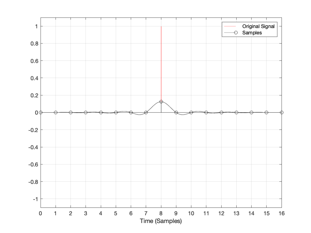
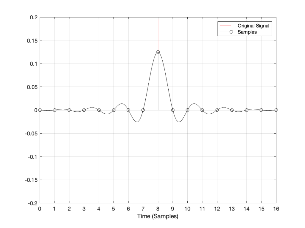
Let’s say that you have an analogue signal that consists of silence and one almost-infinitely short click that is converted to LPCM digital audio. Remember that this click goes through the anti-aliasing low-pass filter, and then gets sampled at some time. Let’s also say that, by some miracle of universal alignment of planets and stars, that click happened at exactly the same time as the sample was measured (we’ll pretend that this is a big deal and I won’t suggest otherwise for the rest of this posting). The result could look like Figure 1.
Figure 1: A click in the analogue domain (red) sampled and encoded as a digital signal (black circles). The analogue output of the digital system will be the black line
If I zoom in on Figure 1 vertically, it looks like the plot in Figure 2.
Figure 2: A vertical zoom of Figure 1.
There are at least three things to notice in these plots.
Since the click happened at the same time as a sample, that sample value is high.
Since the click happened at the same time as a sample, all other sample values are 0.
Once the digital signal is converted back to analogue later (shown as the black line) the maximum point in the signal will happen at exactly the same time as the click
I won’t talk about the fact that the maximum sample value is lower than the original click yet… we’ll deal with that later.
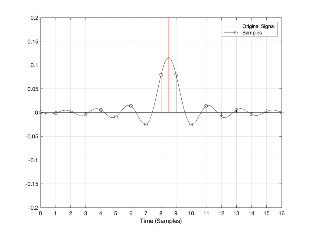
Now, what would happen if the click did not occur at the same time as the sample time? For example, what if the click happened at exactly the half-way point between two samples? This result is shown in Figure 3.
Figure 3: The click happened half-way in time between two samples.
Notice now that almost all samples have some non-zero value, and notice that the two middle samples (8 and 9) are equal. This means that when the signal is converted to analogue (as is shown with the black line) the time of maximum output is half-way between those two samples – at exactly the same time that the click happened.
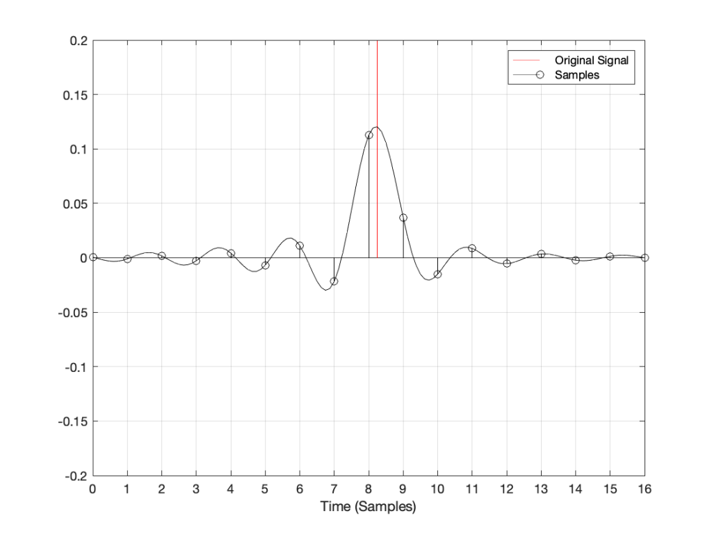
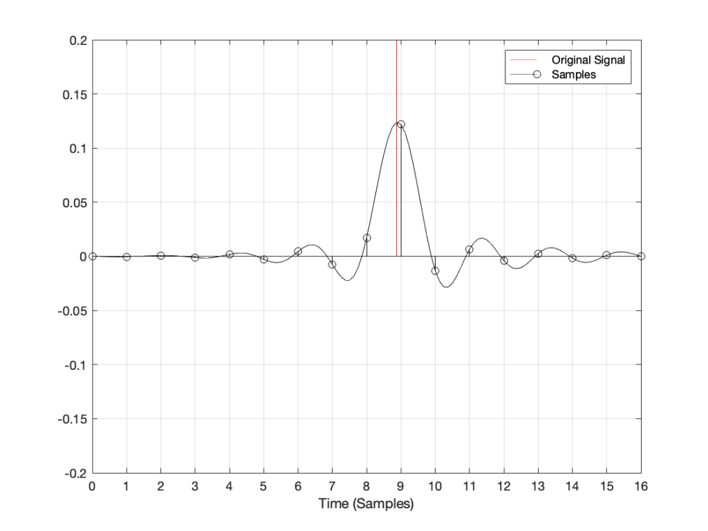
Let’s try some more:
Figure 4: The click happened sometime between two samplesFigure 5: The click happened some other time between two samples.
I could keep doing this all night, but there’s no point. The message here is, no matter when in time the click happened, the maximum output of the digital signal, after it’s been converted back to analogue, happens at exactly the same time.
But, you ask, what about all that “temporal smearing” – the once-pristine click has been reduced to a long wave that extends in time – both forwards and backwards? Waitaminute… how can the output of the system start a wave before something happened?
Okay, okay…. calm down.
Firstly, I’ve made this example using only one type of anti-aliasing filter, and only one type of reconstruction filter. The waveforms I’ve shown here are valid examples – but so are other examples… This depends on the details of the filters you use. In this case, I’m using “linear phase” filters which are symmetrical in time. I could have used a different kind of filter that would have looked different – but the maximum point of energy would have occurred at the same time as the click. Because of this temporal symmetry, the output appears to be starting to ring before the input – but that’s only because of the way I plotted it. In reality, there is a constant delay that I have removed before doing the plotting. It’s just a filter, not a time machine.
Secondly, the black line is exactly the same signal you would get if you stayed in the analogue domain and just filtered the click using the two filters I just mentioned (because, in this discussion, I’m not including quantisation error or dither – they have already been discussed as a separate topic…) so the fact that the signal was turned into “digital” in between was irrelevant.
Thirdly, you may still be wondering why the level of the black line is so low compared to the red line. This is because the energy is distributed in time – so, in fact, if you were to listen to these two clicks, they’d sound like they’re the same level. Another way to say it is that the black line shows exactly the same as if the red curve was band-limited. The only thing missing is the upper part of the frequency band. (You may notice that I have not said anything about the actual sampling rate in any of this posting, because it doesn’t matter – the overall effect in the time domain is the same.)
Fourthly, hopefully you are able to see now that an auditory event that happens between two samples is not thrown away in the conversion to digital. Its timing information is preserved – only its frequency is band-limited. If you still don’t believe me, go listen to a digital recording (which is almost all recordings today) of a moving source – anything moving more than 7 mm will do*. If you can hear clicks in the sound as the source moves, then I’m wrong, and the arrival time of the sound is quantising to the closest sample. However, you won’t hear clicks (at least not because the source is moving), so I’m not wrong. Similarly, if digital audio quantised audio events to the nearest sample, an interpolated delay wouldn’t work – and since lots of people use “flanger” and “phaser” effects on their guitar solos with their weekend garage band, then I’m still right…
The conclusion
Hopefully, from now on, if you are having an argument about high resolution audio, and the person you’re arguing with says “but what about the timing information!? It’s lost at 44.1 kHz!” The correct response is to state (as calmly as possible) “BullS#!T!!”
Rant over.
* I said “7 mm” because I’m assuming a sampling rate of 48 kHz, and a speed of sound of 344 m/s. This means that the propagation distance in air is 344/48000 = 0.0071666 m per sample. In other words, if you’re running a 48 kHz signal out of a loudspeaker, the amplitude caused by a sample is 7 mm away when the next sample comes out.
Thought another way, if you have a stereo system, and your left loudspeaker is 7 mm further away from you than your right loudspeaker, at 48 kHz, you can delay the right loudspeaker by 1 sample to re-align the times of arrival of the two signals at the listening position.
We’ve already seen that nothing can exist in the audio signal above the Nyquist frequency – one half of the sampling rate. But that’s the audio signal, what happens to filters? Basically, it’s the same – the filter can’t modify anything above the Nyquist frequency. However, the problem is that the filter doesn’t behave well to everything up to the Nyquist and then stop, it starts misbehaving long before that…
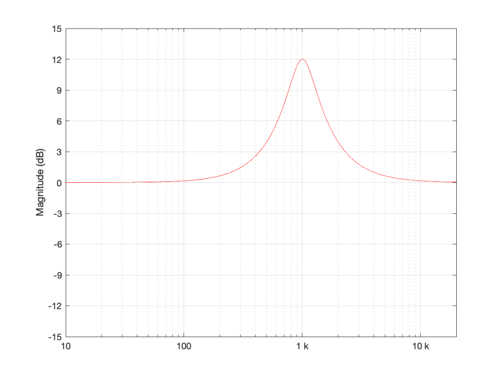
Let’s make a simple filter: a peaking filter where Fc=1 kHz, Gain = 12 dB, and Q=1. The magnitude response of that filter is shown in Figure 1.
Figure 1: Magnitude response of a filter with Fc=1 kHz, Gain = 12 dB, and Q=1
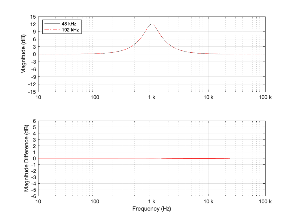
What happens if we implement this filter with a sampling rate of 48 kHz and 192 kHz, and then look at the difference between the two? This is shown in Figure 2.
Figure 2: TOP: The black curve shows the same filter from Figure 1, implemented using a biquad running at 48 kHz. The red dotted line shows the same filter, implemented using a biquad running at 192 kHz. BOTTOM: the difference between the two up to the Nyquist frequency of the 48 kHz system. (there’s almost no difference)
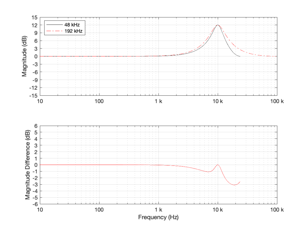
As you can see in Figure 2, the filter, centred at 1 kHz, is almost identical when running at 48 kHz and 192 kHz. So far so good. Now, let’s move Fc up to 10 kHz, as shown in Figure 3.
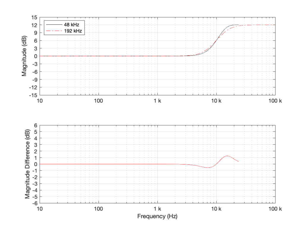
Figure 3: TOP: The black curve shows the magnitude response of a filter with Fc=10 kHz, Gain = 12 dB, and Q=1, implemented using a biquad running at 48 kHz. The red dotted line shows the same filter, implemented using a biquad running at 192 kHz. BOTTOM: the difference between the two up to the Nyquist frequency of the 48 kHz system.
Take a look at the black plot on the top of Figure 3. As you can see there, the 48 kHz filter has a gain of 0 dB at 24 kHz – the Nyquist frequency. Looking at the red dotted line, we can see that the actual magnitude of the filter should have been more than +3 dB. Also, looking at the red line in the bottom plot, which shows the difference between the two curves, the 48 kHz filter starts deviating from the expected magnitude down around 1 kHz already.
So, if you want to implement a filter that behaves as you expect in the high frequency region, you’ll get better results easier with a higher sampling rate.
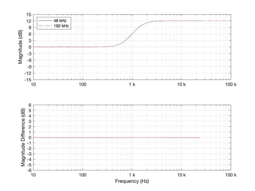
However, do not jump to the conclusion that this also means that you can’t implement a boost in high frequencies. For example, take a look at Figure 4, which shows a high shelving filter where Fc = 1 kHz, Gain = 12 dB and Q = 0.707.
Figure 4: High shelving filter where Fc = 1 kHz, Gain = 12 dB and Q = 0.707.
As you can see in the bottom plot in Figure 4, the two filters in this case (one running at 48 kHz and the other at 192 kHz) have almost identical magnitude responses. (Actually, there is a small difference of about 0.013 dB…) However, if the Fc of the shelving filter moves to 10 kHz instead (keeping the other two parameters the same) then things do get different.
Figure 5: High shelving filter where Fc = 10 kHz, Gain = 12 dB and Q = 0.707.
As can be seen there, there is a little over a 1 dB difference in the two implementations of the same filter.
Some comments:
I’m not going to get into exactly why this happens. If you want to learn about it, look up “bilinear transform”. The short version of the issue is that these filters are designed to work in a system with an infinite sampling rate and bandwidth (a.k.a. analogue), but the band-limiting of an LPCM digital system makes things misbehave as you get near the Nyquist frequency.
This does not mean that you cannot design a filter to get the response you want up to the Nyquist frequency. If you look at the red dotted curve in Figure 3 and call that your “target”, it is possible to build a filter running at 48 kHz that achieves that magnitude response. It’s just a little more complicated that calculating the gain coefficients for the biquad and pretending as if you were normal. However, if you’re a DSP Engineer and your job is making digital filters (say, for correcting tweeter responses in a digitally active loudspeaker, for example) then dealing with this issue is exactly what you’re getting paid for – so you don’t whine about it being a little more complicated.
The side-effect of this, however, is that, if you’re a lazy DSP engineer who just copies-and-pastes your biquad coefficient equations from the Internet, and you just plug in the parameters you want, you aren’t necessarily going to get the response that you think. Unfortunately, this is not uncommon, so it’s not unusual to find products where the high-frequency filtering measures a little strangely, probably because someone in development either wasn’t meticulous or didn’t know about this issue in the first place.