Excruciating minutiae: Part 2

In Part 1, I talked about how an audio signal is quantised, and how the world that the quantised signal lives in is slightly asymmetrical.

Let’s stay in a 3-bit world (to keep things comprehensible on a human scale) and do some recreational quantisation. We’ll start by making a sine wave with a peak amplitude of 1. This means that the total range will be ±1.
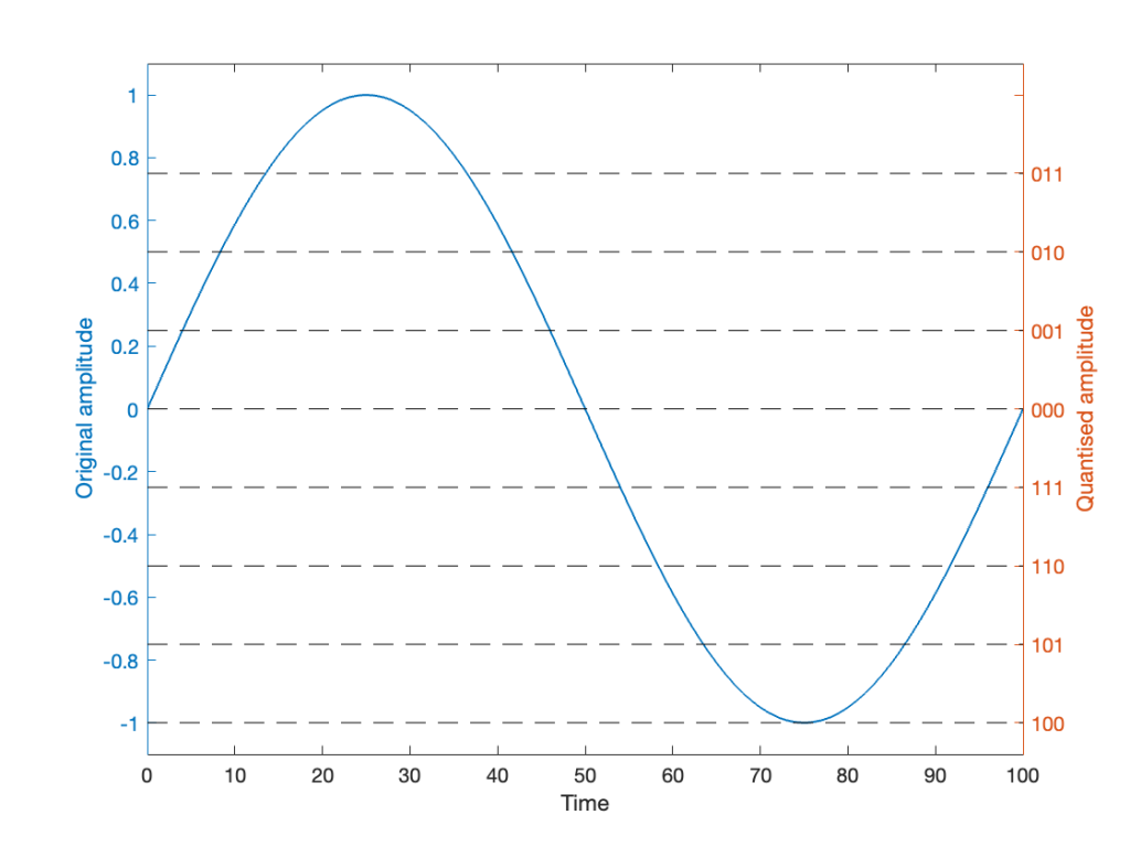
Figure 1. A sine wave with an amplitude of 1.

Notice that I put two scales on the plot in Figure 1. On the left, we have the “floating point” amplitude scale. On the right, we have the 8 quantisation levels.

If we are a bit dumb, and we just quantise that sine wave directly, making sure that I’ve aligned the scaling to use ALL possible quantisation values, we get the result in Figure 2.
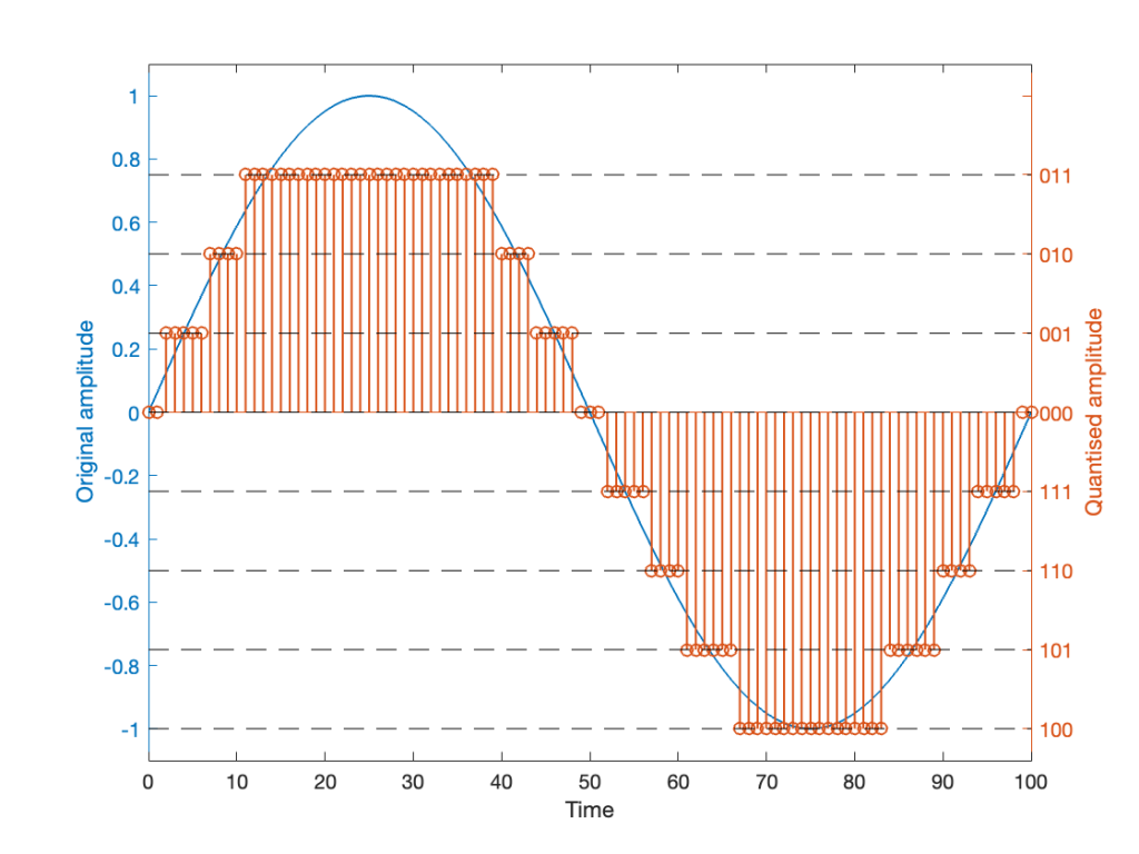
Figure 2. The original signal in blue and the quantised representation in red.

Notice that, because the original signal is symmetrical (with respect to positive and negative amplitudes) but the quantisation steps are not, we wind up getting a different result for the positive values than the negative values. In other words, after quantisation, I’ve clipped the positive peaks of the original signal.

Okay, so this is a dumb way to do this. A slightly less dumb way is to adjust the scaling so that the original wave does not use all possible quantisation values, as shown in Figure 3.
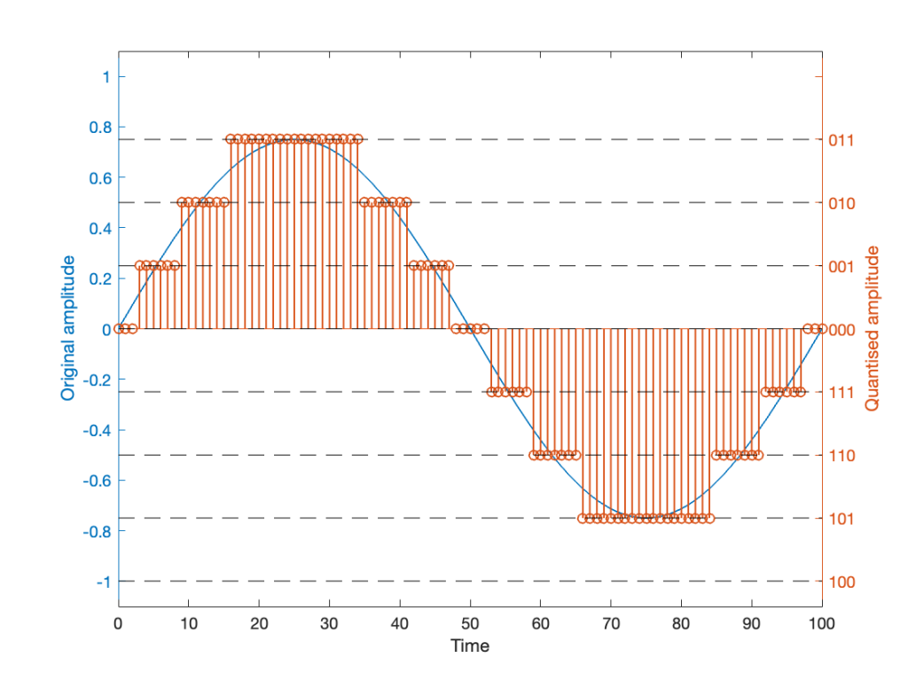
Figure 3.

Notice that I’ve set the sine wave to a slightly lower level, so that it rounds to the top-most positive quantisation level, but this means that it doesn’t use the lowest negative quantisation level. If we’re being really picky, I could have made the sine wave just a little higher in amplitude: by 1/2 of a quantisation step, and the quantised result would still not have clipped asymmetrically.

Dither

As you can see in Figures 2 and 3 above, just taking a signal and quantising it generates an error. The more bits you have in the word length, the more quantisation levels you have, and the smaller the error. However, that error will always be correlated with the signal somehow, and as a result, it’s distortion, which is easy to learn to hear.

If, however, we add a little noise to the signal before we quantise it, then we can randomise the error, which changes the error from producing distortion to a constant signal-independent noise floor. Since the noise makes the quantiser appear to be indecisive, we call it dither.

The easiest (and possibly best) way to do this is to create white noise with a triangular probability distribution function and a peak-to-peak amplitude of ± 1 quantisation level. I’ll explain what that last sentence means in Part 3 of this series.

If we do this, then we

  • take the signal
  • add a little noise to it
  • quantise it

and the result might look like Figure 4.
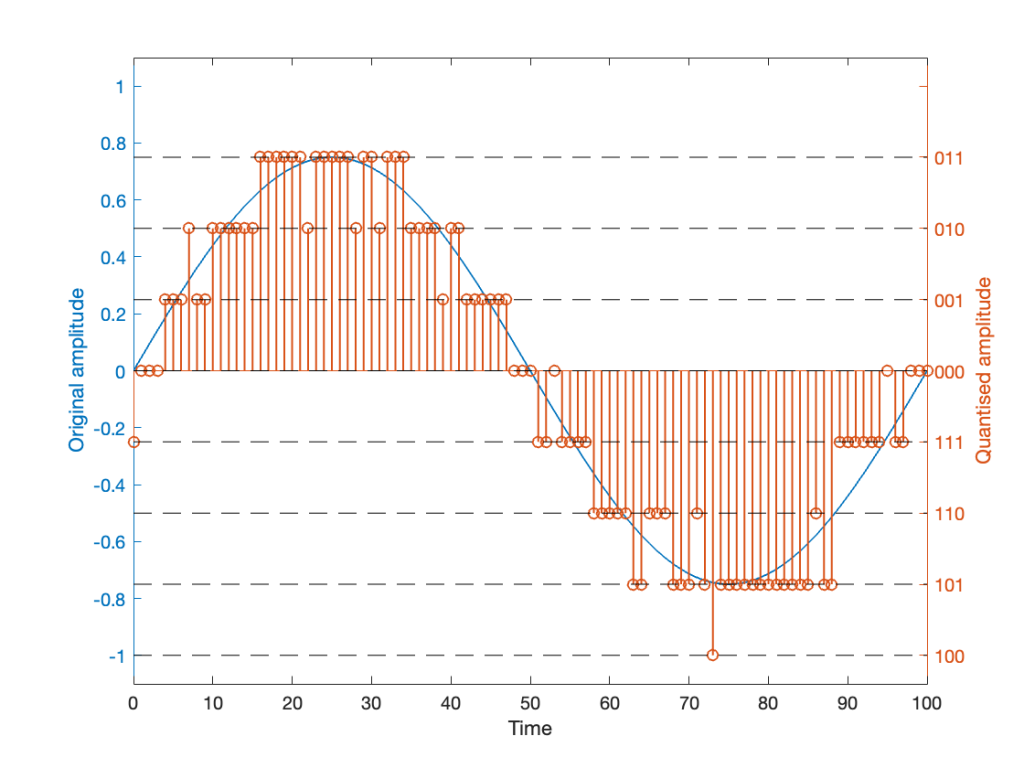
Figure 4.

It should be easy to see that we still have quantisation, and also that I’ve added some random element to the signal.

However, let’s look at the mistake I made in Figure 4. The noise that was added to the signal has an amplitude of ±1 quantisation level. So, we should see cases where the signal looks like it should be rounding to the closest level, but it might be either 1 above or 1 below. (For example, take a look at Time = 70, 71, and 72 as an example of this.)

However, take a look around Time = 20 to 30. Notice that the original signal is close to the top quantisation level. This means that, although a negative value in the dither in those samples can bring the quantisation level down, a positive value cannot bring it up because we don’t have any room for it. This will, again, result in a small amount of asymmetrical clipping. This is a VERY small amount. (Remember that, in the real world we’re probably using 216 (= 65,536) or 224 (= 16,777,216) quantisation values, not 23 (= 8).

So, if we’re going to avoid this clipping, we need to adjust the scaling of the signal once more, as shown in Figure 5.
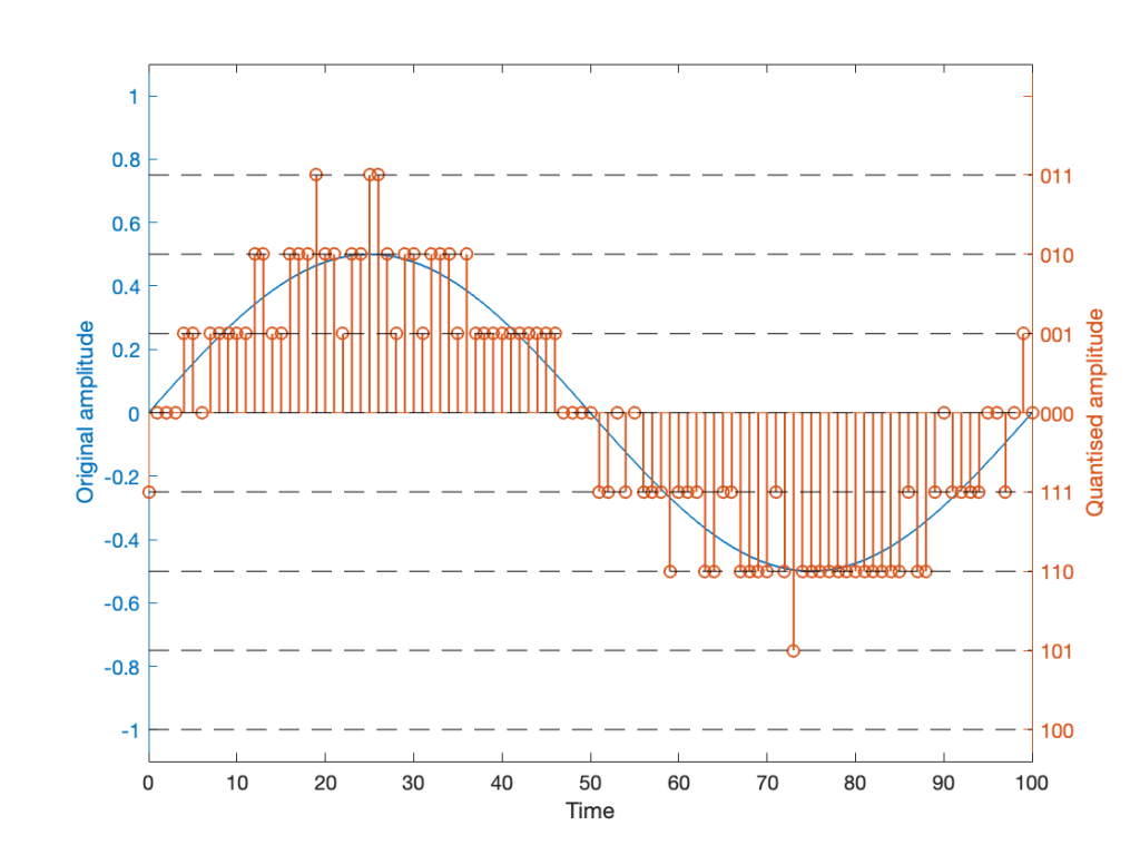
Figure 5.

This shows a signal that is scaled so that, without dither, it would round to one level away from the top-most quantisation level. When you add the dither, it can go up to that top quantisation level. (In fact, I happened to use the same dither signal for Figures 4 and 5. The only difference is the scaling of the signal.)

Now, I know that if you’re not used to looking at 3-bit signals, and/or if dither is a new concept, the red signal in Figure 5 might make you a little upset. However (and you have to believe me on this…) this is the correct way to encode digital audio. Just because it looks crazy doesn’t mean that it is.

NB: The math

If you want to make the plots above, here’s a simplified version of the math to try it out. Note: I live in a world where a % symbol precedes a comment.

Some Constants

Bitdepth = 3
Fs = 100 % sampling rate in Hz
Fc = 1 % frequency of the sine wave in Hz
TimeInSamples = [0:Fs] % This will make the TimeInSamples all of the integer values from 0 to Fs (therefore, 1 second of audio)

Figure 1

Signal = sin(2 * pi * Fc/Fs * TimeInSamples)

Figure 2

ScaleUp = 2^(Bitdepth-1)
ScaleDown = 2^(Bitdepth-1)

QuantisedSignal = round(Signal * ScaleUp) / ScaleDown;

% Then apply a clipper to remove the top quantisation level.
% You can do this yourself.

Figure 3

ScaleUp = 2^(Bitdepth-1)-1
ScaleDown = 2^(Bitdepth-1)

QuantisedSignal = round(Signal * ScaleUp) / ScaleDown;

Figure 4

ScaleUp = 2^(Bitdepth-1)-1
ScaleDown = 2^(Bitdepth-1)
TpdfDither = rand(LengthOfSignal) - rand(LengthOfSignal)

QuantisedDitheredSignal = round(Signal * ScaleUp + TpdfDither) / ScaleDown;
% Then apply a clipper to remove the top quantisation level.

Figure 5

ScaleUp = 2^(Bitdepth-1)-2
ScaleDown = 2^(Bitdepth-1)
TpdfDither = rand(LengthOfSignal) - rand(LengthOfSignal)

QuantisedDitheredSignal = round(Signal * ScaleUp + TpdfDither) / ScaleDown;


Excruciating minutiae: Part 1

This past week I found a very small oddity in the behaviour of one of the functions in Matlab. This led me down a rabbit hole that I’m still following, but the stuff I’ve learned along the way has proven to be interesting.

The summary

The short version of the story is that I made a test tone which consisted of a sine wave that had a frequency that matched an FFT bin centre so that I could test a thing. In order to get the sine wave through the thing, I had to export the audio signal as something the thing could play. So, I exported it as both a .wav and a .flac file, both with 24-bit word lengths and matching sampling rates.

Once the two signals came back from the thing, they looked different on an FFT analysis. Not very different, but different enough to raise questions. So, I ran the FFT on the .wav and .flac files that I created to do the test and found out that THEY were different, which I didn’t expect, because I know that FLAC is lossless.

The question that came up first was “why are they different?”, and that was just the entrance to the rabbit hole.

The long version

In order to explain what happened, we have to following some advice given by Carl Sagan who said

‘If you wish to make an apple pie from scratch, you must first invent the universe.’

We won’t invent the universe, but we’re going to dig down into the basics of LPCM digital audio in order to come back up to talk about where I wound up last Thursday.

Quantisation

Linear Pulse Code Modulation (LPCM) is a way of encoding signals (like an audio signal) by saving the waveform as a series of measurements of the instantaneous amplitude. However, when you do this, you can’t have a measurement with an infinite resolution, so you have to round off the value to the nearest one you can encode. This is just like measuring something with a ruler that has millimetres marked on it. You can’t really measuring something with a precision of less than the nearest millimetre, so you round off the value to something you know. Whether or not that’s good enough depends on what the measurement is for.

In LPCM digital audio, we call the steps that you can round the values to ‘quantisation levels’ because you’re dividing up the amplitude into discrete quanta. Since the values of those quantisation levels are stored or transmitted using a binary number (containing only 0s and 1s), the number of quantisation levels is a power of 2. For example, if you have a 16-bit (bit = Binary digIT) value, then you can count from

0000 0000 0000 0000 = 0
to
1111 1111 1111 1111 = 216 = 65,536

However, since audio signals go above and below 0 (we need to represent positive and negative values) we need a way to split up those options above (a range of 0 to 65,536) to do this.

Let’s take a simple example with a 3-bit long word. Since there are 3 bits, we have 23 = 8 quantisation levels. It would be nice if 000 in the binary representation referred to a signal value of 0, like this:

Figure 1.

All we need to do now is to figure out what binary values to put on the other quantisation levels. To do this, we use a system like the one shown in Figure 2.

Figure 2.

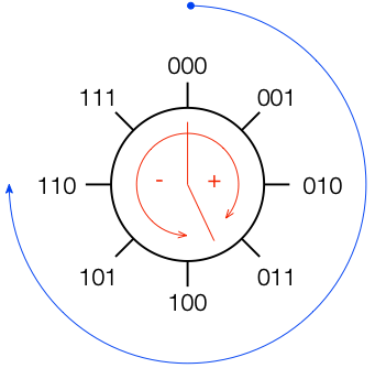
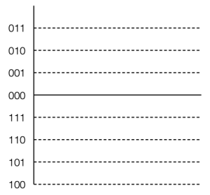
If you start at the top, and follow the blue circular arrow going clockwise, you count from 000 ( = 0) all the way to 111 (= 7). However, if you look at the red arrows, you can see that we can assign the binary values to the positive and negative quantisation levels by looking at the circle clockwise for positive values and counter-clockwise for negative ones. This means that we wind up with the assignments shown in Figure 3.

Figure 3.

This way of using ‘wrapping’ the values around the circle into number assignments on a one-dimensional (in this case, vertical) scale is called a ‘two’s complement’ method.

There are two nice things about this system:

  • the middle value of 0 is assigned an actual value of 0, which makes sense to us humans
  • the first bit (digit) in the binary value tells you whether the level is positive (if it’s a 0) or negative (if it’s a 1).

There is at least one slightly annoying thing about this system: it’s asymmetrical. Notice in Figure 3 that there are 3 available positive quantisation levels, but 4 negative ones. This is because we have an even number of values to use (because it’s a power of 2) but one of the values is 0, leaving an odd, and therefore asymmetrical number of remaining values for the non-0 quantisation levels.

This will come back to be a pain in the arse later…

Excursion vs. Frequency

Last week, I was doing a lecture about the basics of audio and I happened to mention one of the rules of thumb that we use in loudspeaker development:

If you have a single loudspeaker driver and you want to keep the same Sound Pressure Level (or output level) as you change the frequency, then if you go down one octave, you need to increase the excursion of the driver 4 times.

One of the people attending the presentation asked “why?” which is a really good question, and as I was answering it, I realised that it could be that many people don’t know this.

Let’s take this step-by-step and keep things simple. We’ll assume for this posting that a loudspeaker driver is a circular piston that moves in and out of a sealed cabinet. It is perfectly flat, and we’ll pretend that it really acts like a piston (so there’s no rubber or foam surround that’s stretching back and forth to make us argue about changes in the diameter of the circle). Also, we’ll assume that the face of the loudspeaker cabinet is infinite to get rid of diffraction. Finally, we’ll say that the space in front of the driver is infinite and has no reflective surfaces in it, so the waveform just radiates from the front of the driver outwards forever. Simple!

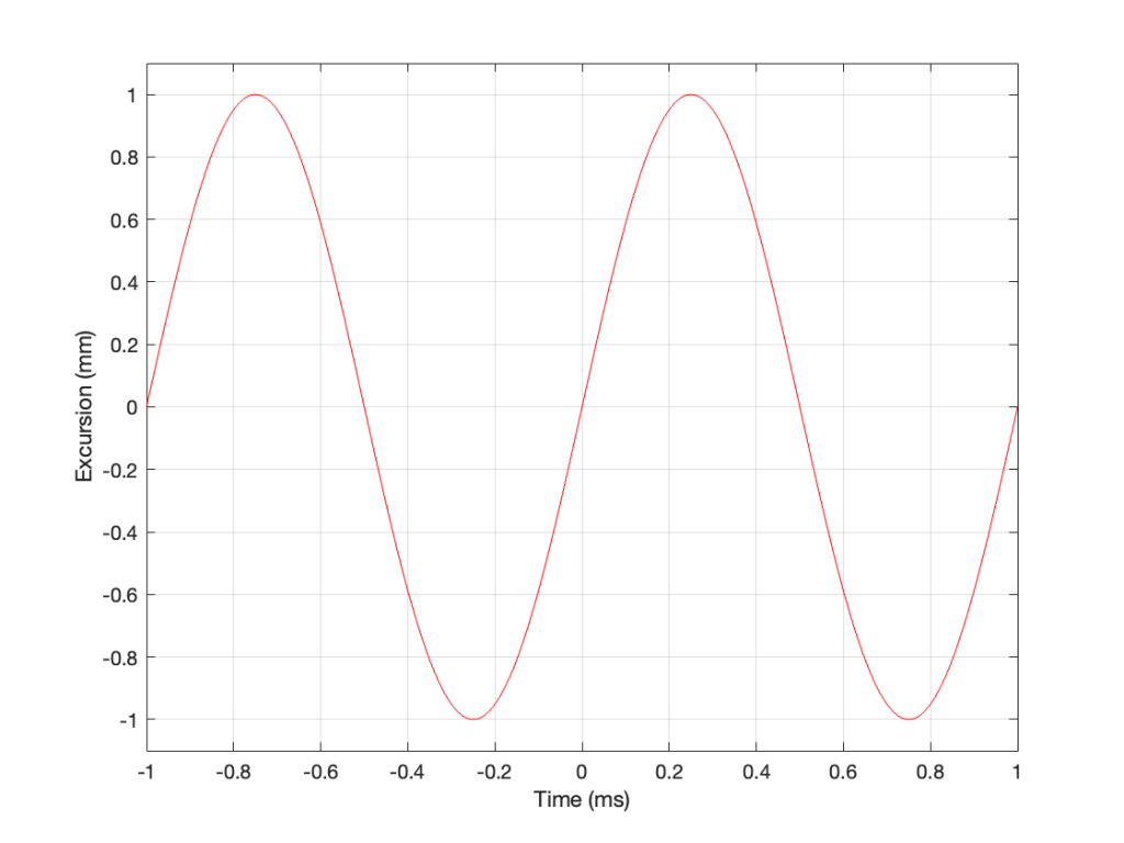
Then, we’ll push and pull the loudspeaker driver in and out using electrical current from a power amplifier that is connected to a sine wave generator. So, the driver moves in and out of the “box” with a sinusoidal motion. This can be graphed like this:

Figure 1: The excursion of a loudspeaker driver playing a 1 kHz sine wave at some output level.

As you can see there, we have one cycle per millisecond, therefore 1000 cycles per second (or 1 kHz), and the driver has a peak excursion of 1 mm. It moves to a maximum of 1 mm out of the box, and 1 mm into the box.

Consider the wave at Time = 0. The driver is passing the 0 mm line, going as fast as it can moving outwards until it gets to 1 mm (at Time = 0.25 ms) by which time it has slowed down and stopped, and then starts moving back in towards the box.

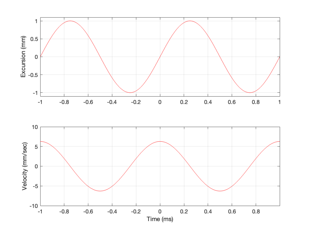
So, the velocity of the driver is the slope of the line in Figure 1, as shown in Figure 2.

Figure 2: The excursion and velocity of the same loudspeaker driver playing the same signal.

As the loudspeaker driver moves in and out of the box, it’s pushing and pulling the air molecules in front of it. Since we’ve over-simplified our system, we can think of the air molecules that are getting pushed and pulled as the cylinder of air that is outlined by the face of the moving piston. In other words, its a “can” of air with the same diameter as the loudspeaker driver, and the same height as the peak-to-peak excursion of the driver (in this case, 2 mm, since it moves 1 mm inwards and 1 mm outwards).

However, sound pressure (which is how loud sounds are) is a measurement of how much the air molecules are compressed and decompressed by the movement of the driver. This is proportional to the acceleration of the driver (neither the velocity nor the excursion, directly…). Luckily, however, we can calculate the driver’s acceleration from the velocity curve. If you look at the bottom plot in Figure 2, you can see that, leading up to Time = 0, the velocity has increased to a maximum (so the acceleration was positive). At Time = 0, the velocity is starting to drop (because the excursion is on its was up to where it will stop at maximum excursion at time = 0.25 ms).

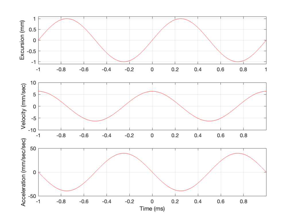
In other words, the acceleration is the slope of the velocity curve, the line in the bottom plot in Figure 2. If we plot this, it looks like Figure 3.

Figure 3: The excursion, velocity and acceleration of the same loudspeaker driver playing the same signal.

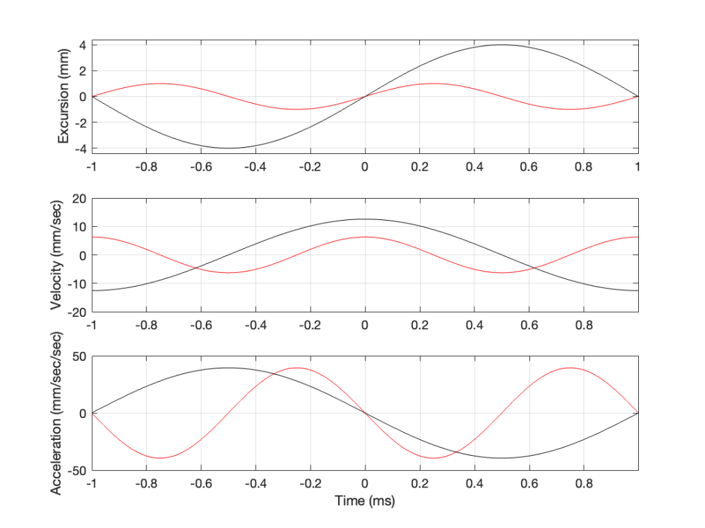
Now we have something useful. Since the bottom plot in Figure 3 shows us the acceleration of the driver, then it can be used to compare to a different frequency. For example, if we get the same driver to play a signal that has half of the frequency, and the same excursion, what happens?

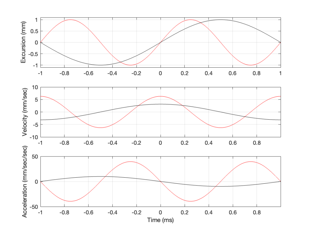
Figure 4: Comparing the excursion, velocity and acceleration of the same loudspeaker driver playing two different signals with the same excursion. (The red line is the same in Figure 4 as in Figure 3.)

In Figure 4, two sine waves are shown: the black line is 1/2 of the frequency of the red line, but they both have the same excursion. If you take a look at where both lines cross the Time = 0 point, then you can see that the slopes are different: the red line is steeper than the black. This is why the peak of the red line in the velocity curve is higher, since this is the same thing. Since the maximum slope of the red line in the middle plot is higher than the maximum slope of the black line, then its acceleration must be higher, which is what we see in the bottom plot.

Since the sound pressure level is proportional to the acceleration of the driver, then we can see in the top and bottom plots in Figure 4 that, if we halve the frequency (go down one octave) but maintain the same excursion, then the acceleration drops to 25% of the previous amount, and therefore, so does the sound pressure level (20*log10(0.25) = -12 dB, which is another way to express the drop in level…)

This raises the question: “how much do we have to increase the excursion to maintain the acceleration (and therefore the sound pressure level)?” The answer is in the “25%” in the previous paragraph. Since maintaining the same excursion and multiplying the frequency by 0.5 resulted in multiplying the acceleration by 0.25, we’ll have to increase the excursion by 4 to maintain the same acceleration.

Figure 5: Comparing the excursion, velocity and acceleration of the same loudspeaker driver playing two different signals at two different excursions. Notice that some of the vertical scales in the plots have changed. (The red line is the same in Figure 5 as in Figures 4 and 3.)

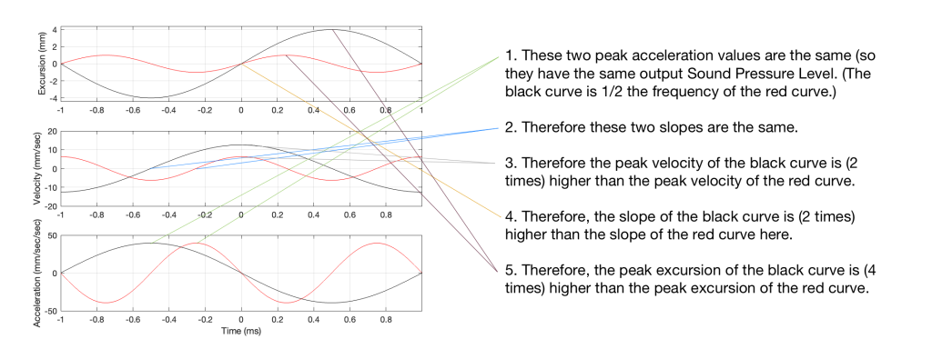
Looking at Figure 5: The black line is 1/2 the frequency of the red line. Their accelerations (the bottom plots) have the same peak values (which means that they produce the same sound pressure level). This, means that the slopes of their velocities are the same at their maxima, which, in turn, means that the peak velocity of the black line (the lower frequency) is higher. Since the peak velocity of the black line is higher (by a factor of 2) then the slope of the excursion plot is also twice as steep, which means that the peak of the excursion of the black line is 4x that of the red line. All of that is explained again in Figure 6.

Figure 6. A repeat of Figure 5 with some explanations that (hopefully) help.

Therefore, assuming that we’re using the same loudspeaker driver, we have to increase the excursion by a factor of 4 when we drop the frequency by a factor of 2, in order to maintain a constant sound pressure level.

However, we can play a little trick… what we’re really doing here is increasing the volume of our “cylinder” of air by a factor of 4. Since we don’t change the size of the driver, we have to move it 4 times farther.

However, the volume of a cylinder is

π r2 * height

and we’re just playing with the “height” in that equation. A different way would be to use a different driver with a bigger surface area to play the lower frequency. For example, if we multiply the radius of the driver by 2, and we don’t change the excursion (the “height” of the cylinder) then the total volume increases by a factor of 4 (because the radius is squared in the equation, and 2*2 = 4).

Another way to think of this: if our loudspeaker driver was a square instead of a circle, we could either move it in and out 4 times farther OR we would make the width and the length of the square each twice as big to get the a cube with the same volume. That “r2” in the equation above is basically just the “width * length” of a circle…

This is why woofers are bigger than tweeters. In a hypothetical world, a tweeter can play the same low frequencies as a woofer – but it would have to move REALLY far in and out to do it.

Transistors vs. Tubes/Valves: A good little reminder

I was leafing through some old editions of Wireless World magazine this week and came across an article in the July, 1968 issue called “Computing Distortion: Method for low-power transistor amplifiers” by L. B. Arguimbau and D.M. Fanger.

I was immediately intrigued by the first sentence, which read:

Unlike those of thermionic valves, the non-linearities in junction transistors for low collector currents are highly uniform and predictable, hardly differing from one transistor to another.

Now, as an “audio professional”, I’m very used to seeing the “±” sign in data sheets. Any production line of anything has some tolerance limits within which the product will fall.

For example, the (on-axis, where applicable) magnitude response of a loudspeaker or headphone is typically spec’ed something like ± 3 dB within some frequency range. This would mean that, at some frequency within that range, when measured under identical conditions, two “identical” products (e.g. with the same brand and model name) might be as much as 6 dB apart.

For different devices and components inside those devices, the tolerance values are different.

This is why, for example, when I read that someone says “headphone model A has more bass than headphone model B”, I know that if you included the missing information, it would actually read “my sample of headphone model A has more bass than my sample of headphone model B”.

However, when it comes down to the component level, I’m used to seeing tighter tolerances. Of course, if you save money on resistors, they might be within 20% of the stated value. However, if I look at the specs of a decent DAC (which, in my case, is a chip that would be used inside a product – not a big DAC-in-a-box that sits on your desk), I’m used to seeing numbers like < ±1 dB within pragmatically usable frequency ranges.

Since I’m only a young person, I’ve only really worked with transistor-based equipment, both when I worked in studios and also since I started working in home audio. So, I’ve always taken it for granted, and never even considered that the distortion characteristics of a transistor would vary from one to another. This is because, as the article from 1968 states: they don’t… much…

However, I’ve never thought about the (now obvious) possibility that two “identical” tubes/valves will have different distortion behaviour, even at low levels, due to manufacturing differences.

So, the next time someone tells you that this tube amp is better than that tube amp (which I translate in my head to actually mean “I prefer the sound of this tube amp over the sound of that tube amp” since “better” is multi-dimensional with different weightings of the different dimensions by person), remind them that the full sentence should be:

“I prefer My sample of this tube amp with the tubes that are currently in it to that tube amp with the tubes that are currently in it.”

32 is a lot of bits…

Once upon a time, I did a blog posting about why, when we test digital audio systems, we typically use a 997 Hz sine wave instead of a 1000 Hz tone.

The short version of this is the following:

Let’s say that I digitally create a (not-dithered) 1000 Hz sine wave at 0 dB FS in a 16-bit system running at 48 kHz. This means that every second, there are exactly 1000 cycles of the wave, and since there are 48,000 samples per second, this, in turn means that there is one cycle every 48 samples, so sample #49 is identical to sample #1.

So, we are only testing 48 of the possible 2^16 ( = 65,536) quantisation values, right?

Wrong. It’s worse than you think.

If we zoom in a little more, we can see that Sample #1 = 0 (because it’s a sine wave). Sample #25 is also equal to 0 (because 48,000 / 1,000 is a nice number that is divisible by 2).

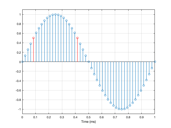
Unfortunately, 48,000 / 1,000 is a nice number that is also divisible by 4. So what? This means that when the sine wave goes up from 0 to maximum, it hits exactly the same quantisation values as it does on the way from maximum back down to 0. For example, in the figure below, the values of the two samples shown in red are identical. This is true for all symmetrical points in the positive side and the negative side of the wave.

Jumping ahead, this means that, if we make a “perfect” 1 kHz sine wave at 48 kHz (regardless of how many bits in the system) we only test a total of 25 quantisation steps. 0, 12 positive steps, and 12 negative ones.

Not much of a test – we only hit 25 out of a possible 65,546 values in a 16-bit system (or 25 out of 16,777,216 possible values in a 24-bit system).

What if I wanted to make a signal that tested ALL possible quantisation values in an LPCM system? One way to do this is to simply make a linear ramp that goes from the lowest possible value up to the highest possible value, step by step, sample by sample. (of course, there are other ways, but it doesn’t matter… we’re just trying to hit every possible quantisation value…)

How long would it take to play that test signal?

First we convert the number of bits to the number of quantisation steps. This is done using the equation 2^bits. So, you get the following results

Number of BitsNumber of Quantisation Steps
1665,536
2416,777,216
324,294,967,296

If the value of each sample has a different quantisation value, and we play the file at the sampling rate then we can calculate the time it will take by dividing the number of quantisation steps by the sampling rate. This results in the following:

Sampling Rate (kHz)16 Bits24 Bits32 Bits
44.11.5 seconds6.4 minutes27.1 hours
481.4 seconds5.8 minutes24.9 hours
88.20.7 seconds3.2 minutes13.5 hours
960.7 seconds2.9 minutes12.4 hours
176.40.4 seconds1.6 minutes6.8 hours
1920.3 seconds1.5 minutes6.2 hours
352.80.2 seconds47.6 seconds3.4 hours
3840.2 seconds43.7 seconds3.1 hours
705.60.1 seconds23.8 seconds1.7 hours
7680.1 seconds21.8 seconds1.6 hours

So, the moral of the story is, if you’re testing the validity of a quantiser in a 32-bit fixed-point system, and you’re not able to do it off-line (meaning that you’re locked to a clock running at the correct sampling rate) you’d either (1) hope that it’s also a crazy-high sampling rate or (2) that you’re getting paid by the hour.

Why I am thinking about this?

I often get asked for my opinion about audio players; these days, network streamers especially, since they’re in style.

Let’s say, for example, that someone asked me to recommend a network streamer for use with their system. In order to recommend this, I need to measure it to make sure it behaves.

One of the tests I’m going to run is to ensure that every sample value on a file is accurately output from the device. Let’s also make it simple and say that the device has a digital output, and I only need to test 3 LPCM audio file formats (WAV, AIFF and FLAC – since those can be relied to give a bit-for-bit match from file to output). (We’ll also pretend that the digital output can support a 32-bit audio word…)

So, to run this test, I’m going to

  • create test files that I described above (checking every quantisation value at all three bit depths and all 10 sampling rates)
  • play them
  • record them
  • and then compare whether I have a bit-for-bit match from input (the original file) to the output

If you add up all the values in the table above for the 10 sampling rates and the three bit depths, then you get to a total of 4.2 DAYS of play time (playing audio constantly 24 hours a day) per file format.

So, say I wanted to test three file formats for all of the sampling rates and bit depths, then I’m looking at playing & recording 12.6 days of audio – and then I can start the analysis.

REALLY‽

Of course this is silly… I’m not going to test a 32-bit, 44.1 kHz file… In fact, if I don’t bother with the 32-bit values at all, then my time per file format drops from 4.2 days down to 23.7 minutes of play time, which is a lot more feasible, but less interesting if I’m getting paid by the hour.

However, it was fun to calculate – and it just goes to show how big a number 2^32 is…

What is a “virtual” loudspeaker? Part 3

#91.3 in a series of articles about the technology behind Bang & Olufsen

In Part 1 of this series, I talked about how a binaural audio signal can (hypothetically, with HRTFs that match your personal ones) be used to simulate the sound of a source (like a loudspeaker, for example) in space. However, to work, you have to make sure that the left and right ears get completely isolated signals (using earphones, for example).

In Part 2, I showed how, with enough processing power, a large amount of luck (using HRTFs that match your personal ones PLUS the promise that you’re in exactly the correct location), and a room that has no walls, floor or ceiling, you can get a pair of loudspeakers to behave like a pair of headphones using crosstalk cancellation.

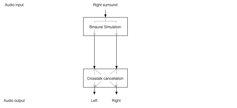
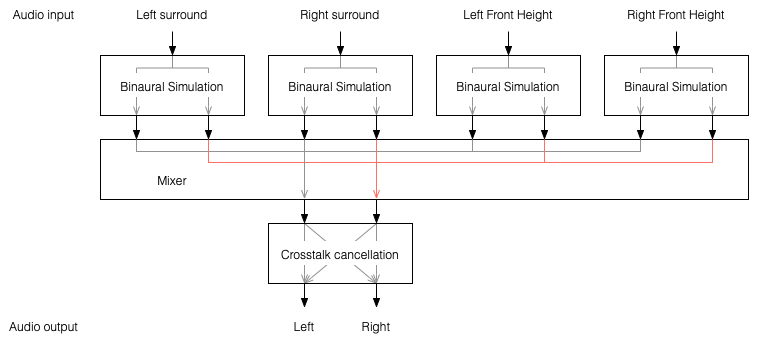
There’s not much left to do to create a virtual loudspeaker. All we need to do is to:

  • Take the signal that should be sent to a right surround loudspeaker (for example) and filter it using the HRTFs that correspond to a sound source in the location that this loudspeaker would be in. REMEMBER that this signal has to get to your two ears since you would have used your two ears to hear an actual loudspeaker in that location.
  • Send those two signals through a crosstalk cancellation processing system that causes your two loudspeakers to behave more like a pair of headphones.
Figure 1: A block diagram of the system described above.

One nice thing about this system is that the crosstalk cancellation is only there to ensure that the actual loudspeakers behave more like headphones. So, if you want to create more virtual channels, you don’t need to duplicate the crosstalk cancellation processor. You only need to create the binaurally-processed versions of each input signal and mix those together before sending the total result to the crosstalk cancellation processor, as shown below.

Figure 2: You only need one crosstalk cancellation system for any number of virtual channels.

This is good because it saves on processing power.

So, there are some important things to realise after having read this series:

  • All “virtual” loudspeakers’ signals are actually produced by the left and right loudspeakers in the system. In the case of the Beosound Theatre, these are the Left and Right Front-firing outputs.
  • Any single virtual loudspeaker (for example, the Left Surround) requires BOTH output channels to produce sound.
  • If the delays (aka Speaker Distance) and gains (aka Speaker Levels) of the REAL outputs are incorrect at the listening position, then the crosstalk cancellation will not work and the virtual loudspeaker simulation system won’t work. How badly is doesn’t work depends on how wrong the delays and gains are.
  • The virtual loudspeaker effect will be experienced differently by different persons because it’s depending on how closely your actual personal HRTFs match those predicted in the processor. So, don’t get into fights with your friends on the sofa about where you hear the helicopter…
  • The listening room’s acoustical behaviour will also have an effect on the crosstalk cancellation. For example, strong early reflections will “infect” the signals at the listening position and may/will cause the cancellation to not work as well. So, the results will vary not only with changes in rooms but also speaker locations.

Finally, it’s worth nothing that, in the specific case of the Beosound Theatre, by setting the Speaker Distances and Speaker Levels for the Left and Right Front-firing outputs for your listening position, then you have automatically calibrated the virtual outputs. This is because the Speaker Distances and Speaker Levels are compensations for the ACTUAL outputs of the system, which are the ones producing the signal that simulate the virtual loudspeakers. This is the reason why the four virtual loudspeakers do not have individual Speaker Distances and Speaker Levels. If they did, they would have to be identical to the Left and Right Front-firing outputs’ values.

What is a “virtual” loudspeaker? Part 2

#91.2 in a series of articles about the technology behind Bang & Olufsen

In Part 1, I talked at how a binaural recording is made, and I also mentioned that the spatial effects may or may not work well for you for a number of different reasons.

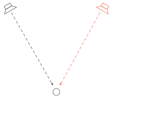
Let’s go back to the free field with a single “perfect” microphone to measure what’s happening, but this time, we’ll send sound out of two identical “perfect” loudspeakers. The distances from the loudspeakers to the microphone are identical. The only difference in this hypothetical world is that the two loudspeakers are in different positions (measuring as a rotational angle) as shown in Figure 1.

Figure 1: Two identical, “perfect” loudspeakers in a free field with a single “perfect” microphone.

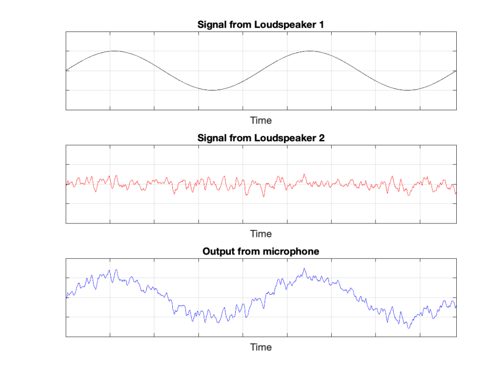
In this example, because everything is perfect, and the space is a free field, then output of the microphone will be the sum of the outputs of the two loudspeakers. (In the same way that if your dog and your cat are both asking for dinner simultaneously, you’ll hear dog+cat and have to decide which is more annoying and therefore gets fed first…)

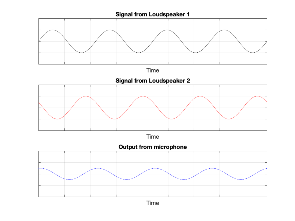
Figure 2: The output from the microphone is the sum of the outputs from the two loudspeakers. At any moment in time, the value of the top plot + the value of the middle plot = the value of the bottom plot.

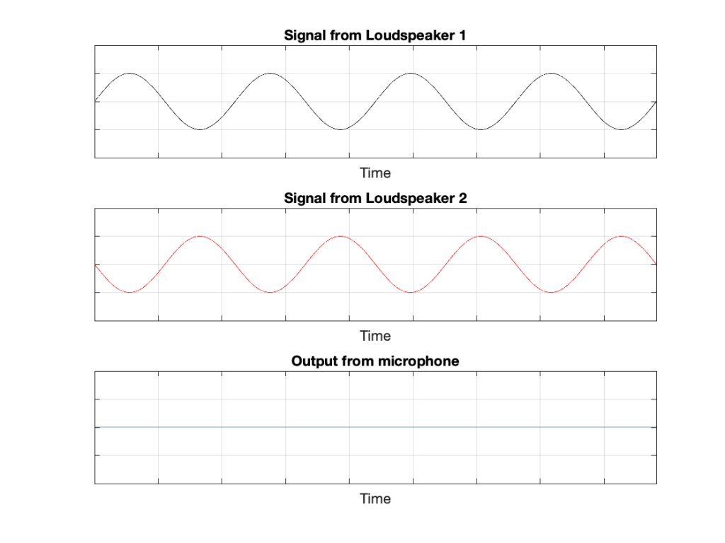
IF the system is perfect as I described above, then we can play some tricks that could be useful. For example, since the output of the microphone is the sum of the outputs of the two loudspeakers, what happens if the output of one loudspeaker is identical to the other loudspeaker, but reversed in polarity?

Figure 3: If the output of Loudspeaker 1 is exactly the same as the output of Loudspeaker 2 except for polarity, then the sum (the output of the microphone) is always 0.

In this example, we’re manipulating the signals so that, when they add together, you nothing at the output. This is because, at any moment in time, the value of Loudspeaker 2’s output is the value of Loudspeaker 1’s output * -1. So, in other words, we’re just subtracting the signal from itself at the microphone and we get something called “perfect cancellation” because the two signals cancel each other at all times.

Of course, if anything changes, then this perfect cancellation won’t work. For example, if one of the loudspeakers moves a little farther away than the other, then the system is broken, as shown below.

Figure 4: A small shift in time in the output of Loudspeaker 2 cases the cancellation to stop working so well.

Again, everything that I’ve said above only works when everything is perfect, and the loudspeakers and the microphone are in a free field; so there are no reflections coming in and ruining everything.

We can now combine these two concepts:

  1. using binaural signals to simulate a sound source in a location (although this would normally be done using playback over earphones to keep it simple) and
  2. using signals from loudspeakers to cancel each other at some location in space as a

to create a system for making virtual loudspeakers.

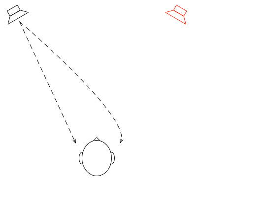
Let’s suspend our adherence to reality and continue with this hypothetical world where everything works as we want… We’ll replace the microphone with a person and consider what happens. To start, let’s just think about the output of the left loudspeaker.

Figure 5: The output of the left loudspeaker reaches both ears with different time/frequency characteristics caused by the HRTF associated with that sound source location.

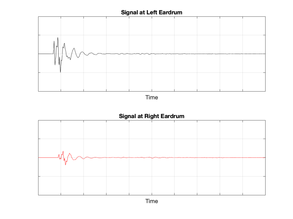
If we plot the impulse responses at the two ears (the “click” sound from the loudspeaker after it’s been modified by the HRTFs for that loudspeaker location), they’ll look like this:

Figure 6: The impulse responses of the HRTFs for a sound source at 30º left of centre.

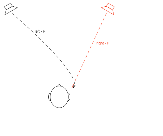
What if were were able to send a signal out of the right loudspeaker so that it cancels the signal from the left loudspeaker at the location of the right eardrum?

Figure 7: What if we could cancel the signal from the left loudspeaker at the right ear using the right loudspeaker?

Unfortunately, this is not quite as easy as it sounds, since the HRTF of the right loudspeaker at the right ear is also in the picture, so we have to be a bit clever about this.

So, in order for this to work we:

  • Send a signal out of the left loudspeaker.
    We know that this will get to the right eardrum after it’s been messed up by the HRTF. This is what we want to cancel…
  • …so we take that same signal, and
    • filter it with the inverse of the HRTF of the right loudspeaker
      (to undo the effects of the HRTF of the right loudspeaker’s signal at the right ear)
    • filter that with the HRTF of the left loudspeaker at the right ear
      (to match the filtering that’s done by your head and pinna)
    • multiply by -1
      (so that it will cancel when everything comes together at your right eardrum)
    • and send it out the right loudspeaker.

Hypothetically, that signal (from the right loudspeaker) will reach your right eardrum at the same time as the unprocessed signal from the left loudspeaker and the two will cancel each other, just like the simple example shown in Figure 3. This effect is called crosstalk cancellation, because we use the signal from one loudspeaker to cancel the sound from the other loudspeaker that crosses to the wrong side of your head.

This then means that we have started to build a system where the output of the left loudspeaker is heard ONLY in your left ear. Of course, it’s not perfect because that cancellation signal that I sent out of the right loudspeaker gets to the left ear a little later, so we have to cancel the cancellation signal using the left loudspeaker, and back and forth forever.

If, at the same time, we’re doing the same thing for the other channel, then we’ve built a system where you have the left loudspeaker’s signal in the left ear and the right loudspeaker’s signal in the right ear; just like a pair of headphones!

However, if you get any of these elements wrong, the system will start to under-perform. For example, if the HRTFs that I use to predict your HRTFs are incorrect, then it won’t work as well. Or, if things aren’t time-aligned correctly (because you moved) then the cancellation won’t work.

on to Part 3

Keep your needle clean

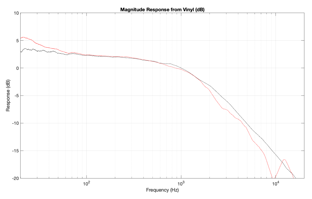
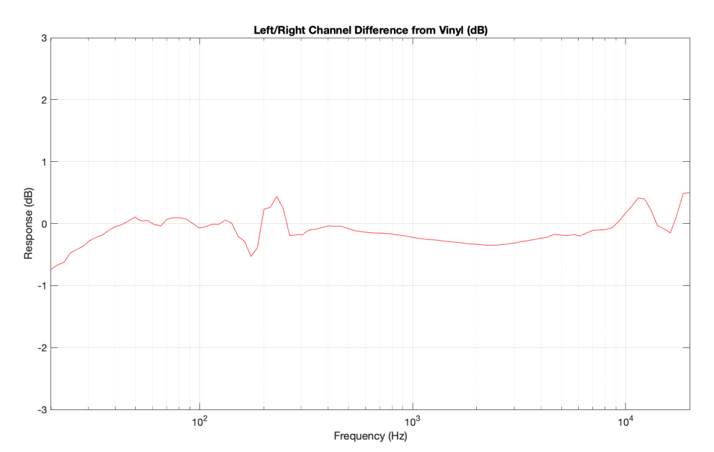
One of my jobs at Bang & Olufsen is to do the final measurements on each bespoke Beogram 4000c turntable before it’s sent to the customer. Those measurements include checking the end-to-end magnitude response, playing from a vinyl record with a sine sweep on it (one per channel), recording that from the turntable’s line-level output, and analysing it to make sure that it’s as expected. Part of that analysis is to very that the magnitude responses of the left and right channel outputs are the same (or, same enough… it’s analogue, a world where nothing is perfect…)

Today, I was surprised to see this result on a turntable that was being inspected part-way through its restoration process :

Taken at face value, this should have resulted in a rejection – or at least some very serious questions. This is a terrible result, with unacceptable differences in output level between the two channels. When I looked at the raw measurements, I could easily see that the left channel was behaving – it was the right channel that was all over the place.

The black curve looks very much like what I would expect to see. This is the result of playing a track that is a sine sweep from 20 Hz to 20 kHz, where the signal below 1 kHz follows the RIAA curve, whereas the signal above 1 kHz does not. This is why, after it’s been filtered using a RIAA preamp, the low frequency portion has a flat response, but the upper frequency band rolls off (following the RIAA curve).

Notice that the right channel (the red curve) is a mess…

A quick inspection revealed what might have been the problem: a small ball of fluff collected around the stylus. (This was a pickup that was being used to verify that the turntable was behaving through the restoration – not the one intended for the final customer – and so had been used multiple times on multiple turntables.)

So, we used a stylus brush to clean off the fluff and ran the measurement again. The result immediately afterwards looked like this:

which is more like it! A left-right channel difference of something like ± 0.5 dB is perfectly acceptable.

The moral of the story: keep your pickup clean. But do it carefully! That cantilever is not difficult to snap.

Filters and Ringing: Part 10

There’s one last thing that I alluded to in a previous part of this series that now needs discussing before I wrap up the topic. Up to now, we’ve looked at how a filter behaves, both in time and magnitude vs. frequency. What we haven’t really dealt with is the question “why are you using a filter in the first place?”

Originally, equalisers were called that because they were used to equalise the high frequency levels that were lost on long-distance telephone transmissions. The kilometres of wire acted as a low-pass filter, and so a circuit had to be used to make the levels of the frequency bands equal again.

Nowadays we use filters and equalisers for all sorts of things – you can use them to add bass or treble because you like it. A loudspeaker developer can use them to correct linear response problems caused by the construction or visual design of the device. They can be used to compensate for the acoustical behaviour of a listening room. Or they can be used to compensate for things like hearing loss. These are just a few examples, but you’ll notice that three of the four of them are used as compensation – just like the original telephone equalisers.

Let’s focus on this application. You have an issue, and you want to fix it with a filter.

IF the problem that you’re trying to fix has a minimum phase characteristic, then a minimum phase filter (implemented either as an analogue circuit or in a DSP) can be used to “fix” the problem not only in the frequency domain – but also in the time domain. IF, however, you use a linear phase filter to fix a minimum phase problem, you might be able to take care of things on a magnitude vs. frequency analysis, but you will NOT fix the problem in the time domain.

This is why you need to know the time-domain behaviour of the problem to choose the correct filter to fix it.

For example, if you’re building a room compensation algorithm, you probably start by doing a measurement of the loudspeaker in a “reference” room / location / environment. This is your target.

You then take the loudspeaker to a different room and measure it again, and you can see the difference between the two.

In order to “undo” this difference with a filter (assuming that this is possible) one strategy is to start by analysing the difference in the two measurements by decomposing it into minimum phase and non-minimum phase components. You can then choose different filters for different tasks. A minimum phase filter can be used to compensate a resonance at a single frequency caused by a room mode. However, the cancellation at a frequency caused by a reflection is not minimum phase, so you can’t just use a filter to boost at that frequency. An octave-smoothed or 1/3-octave smoothed measurement done with pink noise might look like you fixed the problem – but you’ve probably screwed up the time domain.

Another, less intuitive example is when you’re building a loudspeaker, and you want to use a filter to fix a resonance that you can hear. It’s quite possible that the resonance (ringing in the time domain) is actually associated with a dip in the magnitude response (as we saw earlier). This means that, although intuition says “I can hear the resonant frequency sticking out, so I’ll put a dip there with a filter” – in order to correct it properly, you might need to boost it instead. The reason you can hear it is that it’s ringing in the time domain – not because it’s louder. So, a dip makes the problem less audible, but actually worse. In this case, you’re actually just attenuating the symptom, not fixing the problem – like taking an Asprin because you have a broken leg. Your leg is still broken, you just can’t feel it.