
Author: geoff
It’s funny because it’s true…
SVEN: The Surveillance Video Entertainment Network
Max/MSP/Jitter in action!
How much do you like the Beatles?
Enough to bid on this?
Don’t believe everything you see (or hear)
B&O Tech: Intuitive Directivity Plots v.2
#48 in a series of articles about the technology behind Bang & Olufsen loudspeakers
In a past article, I tried to come up with an intuitive way of representing the beam width (or “directivity” – if you’re a geek) of the BeoLab 90. I realised after posting, that there is another way to do this which is used in loudspeaker reviews in some magazines (mostly because it’s the way directivity is plotted by MLSSA). So, I’ve taken the same data as before, and re-plotted it using a “waterfall” function in Matlab. It’s just a different way of looking at the same information – but it might be helpful.
If you’re curious about the details regarding the data itself, this is described here.


Looking for vinyl?

CODEC artefacts that aren’t…
B&O Tech: Product Playlists
#47 in a series of articles about the technology behind Bang & Olufsen loudspeakers
This is just a list of playlists on the Tidal music streaming service that can be used for testing and demonstrating various Bang & Olufsen products.
If you don’t have a Tidal subscription, you can at least see the list of tracks, artists and albums.
Loudspeakers
Televisions
Music Systems
Headphones
B&O Tech: Intuitive Directivity Plots
#46 in a series of articles about the technology behind Bang & Olufsen loudspeakers
I’ve been writing and presenting a lot of information over the past couple of months about the general topic of loudspeaker directivity or “Beam Width” as we call it in the BeoLab 90. One thing that I’ve noticed is that, every time I have to do this in person, I have to explain how to read our directivity plots. This has made me realise that these are not necessarily intuitive to someone that doesn’t look at these kinds of plots (or topographic maps) every day. So, I’ve been working on finding different ways to show the same data. This posting is a first attempt – there will probably be others in the future…
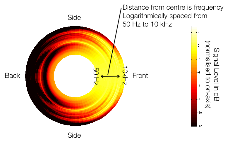
Figure 1, above, shows the idea. We have a loudspeaker, pointing to the right of the screen (towards the word “front”). We measure the magnitude response (more commonly called the “frequency response”) of the loudspeaker on-axis, directly in front of it. Then we rotate the angle of the listening position around the loudspeaker, towards the side. As we do, we measure how much the level changes (usually it gets quieter, but sometimes, at some frequencies and some angles, it gets louder) as a function of angle and frequency. As the angle to the listening position increases, some frequencies will get quiet very quickly, some will not get quiet at all – even when we reach the back of the loudspeaker.
The plot above shows one way to look at this. The inner rings are the low frequencies (in the case of the plots on this webpage, the inner-most ring is 50 Hz) and the further outwards you go, the higher in frequency. The distance between the rings is logarithmic (in other words, by octave) so it makes more sense musically.
If you’re used to looking at the contour plots that I typically show on this site, then take a look at Figure 2 which shows exactly the same data. In this case, it’s plotted as a contour plot (like a topographic map) showing the -3 dB, -6 dB, -9 dB, and -12 dB contours relative to the on-axis response.
BeoLab 90: Beam Width Control: Off
Figures 2 and 3 show the directivity of the BeoLab 90 if you were to disable the Beam Width Control function entirely and just use the front woofer, midrange and tweeter by themselves (and therefore turn off the 15 other loudspeaker drivers in the system. It’s important to note that this is not possible in a production model loudspeaker – we did it as part of the initial measurements of the loudspeaker during the development process.


BeoLab 90: Narrow Beam
As I’ve discussed in other postings, our goal with BeoLab 90’s directivity was two-fold: The first was to have a constant directivity – meaning that it should be the same at all frequencies. The second was that the directivity should be narrow in order to reduce the influence of sidewall reflections. Of course, it should not be too narrow – you don’t want a loudspeaker that you can hear in your left ear, but not your right or “headphones at a distance” as I read on one website.
So, we played around with different target directivity functions during the development process, trying to find a beam width that was not too wide and not too narrow. Figures 4 and 5 aren’t drawings of the actual target for BeoLab 90 – but they’re illustrative of the concept.


The actual directivity of the narrow beam width in BeoLab 90 is plotted in Figures 6 and 7.

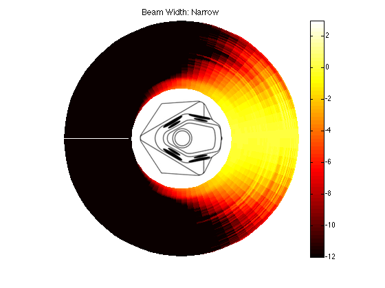
It might also be interesting to compare this to one of BeoLab 90’s competitors from another manufacturer, shown in Figure 8.

BeoLab 90: Wide Beam
Again, we can look at a candidate for a target (but not the target) for the wide beam mode. This is shown in Figures 8 and 9.


The actual directivity of the wide beam is shown in Figures 10 and 11.

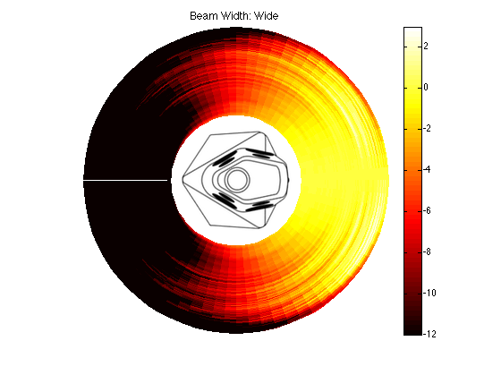
In addition, it might be interesting to compare those plots to the BeoLab 5 directivity, which had similar targets of a constant and wide directivity.


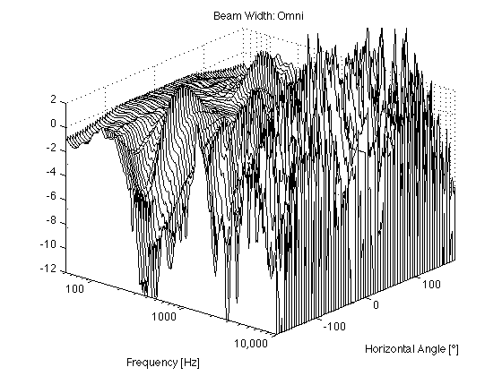
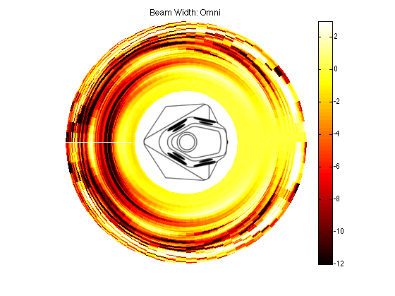
BeoLab 90: Omni Beam
The directivity of BeoLab 90’s Omni mode is shown below in Figures 15 and 16. The lobing caused by the distances between the tweeters is visible in the contour plot, however, as you can see in Figure 16, there is certainly energy being directed in all directions across the entire frequency spectrum. However, the high-frequency lobing, in addition to the beaming in the lower midrange area would indicate that this mode is not appropriate for critical listening…

Some details
The plots above were done in the horizontal plane with a smoothing of 1/12 octave (by semitone).
The measurements on the loudspeakers were done in 73 increments of 5º from -180º to 180º (in other words, we’re actually measuring both sides of the loudspeaker – we don’t just measure one side and assume the directivity is symmetrical.