
Author: geoff
A quick tour of the Struer Museum

Cymatics
Audio economics

Another BeoLab 90 Review – from Axpona

BeoLab 90 review in Germany

One-dimensional answers to a multidimensional question: Part 2
I once read a discussion about microphone placement in an Usenet Forum (it was a long time ago). Someone asked “where is the best place to position the microphones to record a french horn?” Lots of people had opinions, but the answer that I liked most was “that’s like asking ‘where is the best place to stand to take a photo of a mountain?” Of course, that answer might have been too facetious for the person asking the question, but, in my opinion, it was a good analogy. The correct answer, as always, is “it depends” – in this case, on perspective.
Example #1
Take a look at the image below.
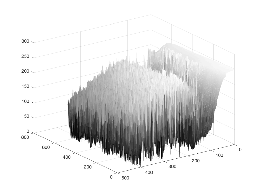
As you can read in the caption, this is a 640 x 480 black and white photo of a fishing boat off the coast of Newfoundland, near where I grew up, on a foggy day. Of course, if I didn’t tell you that, then it would be impossible to know it – but that’s because you’re looking at the “data” (the information in the pixels in the photo) from the wrong place… I’ll rotate the image a little and we’ll try again.
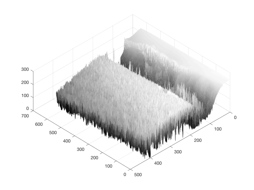
Figure 2 is just a rotation of Figure 1 – we’re still looking at the same photo, but from another direction. It still doesn’t look like a boat… Let’s rotate some more…
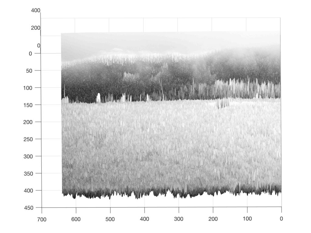
Figure 3 is looking more like something – but there’s still no boat in sight… If you come back to Figure 3 after you look at Figure 4, you’ll recognise the trees on the land, the sky, and the water – you’ll also be able to see where the boat is. But this view of the photo is just off-position enough to scramble the data into being almost unrecognisable. So, let’s rotate the view of the data one last time…
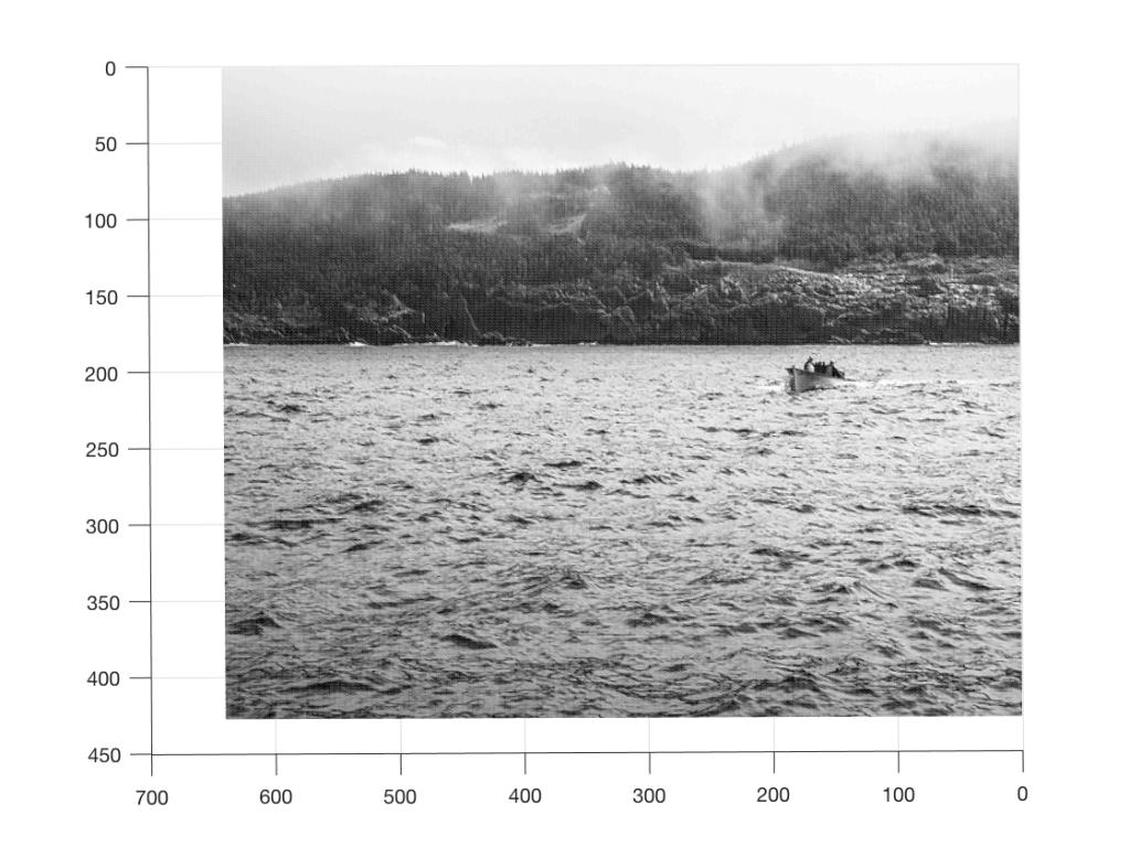
So, what was the point of this, somewhat obscure analogy? It was to try to show that, by looking at the data from only one viewpoint, or one dimension (say, Figure 1, for example), you might arrive at an incorrect interpretation of the data.
Example #2
Watch this video.
In this video, Penn and Teller do the same trick twice. Both times, the trick is impressive, but for two different reasons. This is because your perspective changes. The first time, it’s just a good magic trick – or at least an old one. The second time, you’re impressed because of their skill in executing it. Two different perceptions resulting from two different perspectives.
Example #3
Once-upon-a-time, I taught a course in electroacoustic measurements at McGill University. I remember one class, early in the year, where I started one day by saying “What is a ‘frequency response’?” and one of the students, with a smile on his face replied “The only thing that matters…”
I went through some old data and found a measurement of a loudspeaker. Figure 5, below, shows the magnitude response of a three-way loudspeaker, measured in free-field (therefore, no reflections or influence of the room) at a distance of three meters from the loudspeaker, on-axis to the tweeter.
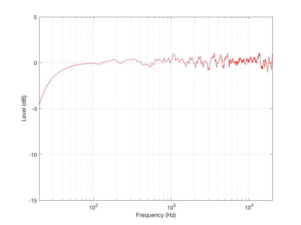
This is just the kind of measurement that you’d see in a magazine… It’s also the kind of measurement that you’d use to make a “frequency response” for a data sheet. This one would read something like “<40 Hz – >20 kHz ±1 dB”, give or take.
However, let’s think about what this really is and whether it actually tells you anything at all… It’s a measurement of the relationship between input voltage to output pressure, in one place in space, at one listening level, with one type of signal (maybe a swept sine wave or an MLS signal, or something else…), at one temperature of the drivers’ voice coils, at one relative humidity level of the air (okay, okay… now I’m getting into excruciating minutæ…)
However, does this tell us anything about how the loudspeaker will sound? Well, yes. If you use it outdoors in a large field and you stand 3 m in front of it and listen to the same signal that was used to do the measurement. If, however, you stand closer, or not directly in front of it, or if you listen to music over time, or if you bring it indoors, this is just one piece of information – perhaps useful, but certainly inadequate…
Let’s look at another measurement of the same loudspeaker
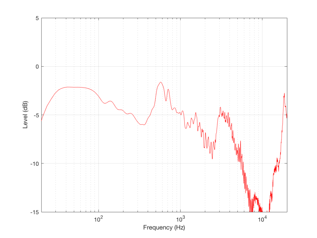
As you can see, this loudspeaker’s magnitude response looks “pretty bad” – or at least “not very flat” off-axis (which implies that I just equated “flat” with “good” – which might not necessarily be correct…).
This is the magnitude response of the signal that this loudspeaker will send out the side while you’re listening to that “nice” flat direct sound. Something like this will hit the side wall and reflect back, different frequencies reflecting with different intensities according to the absorptive properties of the wall, the total distance travelled by the reflection, and the relative humidity (okay, okay …I’ll stop with the humidity references…)
As is obvious in Figure 6, this “sound” is almost completely unlike the “sound” in Figure 5 (assuming that a free-field magnitude response can be translated to “sound” – which is a stretch…)
So, just like in Example 1 and Example 2, by “looking” at the data from another direction, we get some more information that should be used to influence our opinion. The more data from the more perspectives, the better…
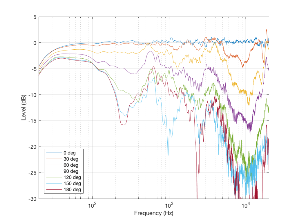
So, we have one measurement that shows that this loudspeaker is “flat” and therefore “good”, in some persons’ opinions. However, we have a bunch of other measurements that prove that this is not enough information. And, if we measure the same loudspeaker at a different listening level, or at a different temperature, or with a different stimulus, we’d probably get a different answer. How different the measurement is is dependent on how different the measurement conditions are.
The “punch line” is that you cannot make any assumptions about how that loudspeaker will sound based on that one measurement in Figure 5 or the “frequency response” information in its datasheet. In fact, it could just be that having that graph in your hand will be worse than having no graphs in your hand, because your eyes might tell you that this speaker should sound good, and they get into a debate with your ears, who might disagree…
So, without more information, that one plot in Figure 5 is just a plot of one parameter – or one dimension – of many. And you can’t make any conclusions based on that.
Or put another way:
An astronomer, a physicist and a mathematician are on a train in Scotland. The astronomer looks out of the window, sees a black sheep standing in a field, and remarks, “How odd. All the sheep in Scotland are black!” “No, no, no!” says the physicist. “Only some Scottish sheep are black.” The mathematician rolls his eyes at his companions’ muddled thinking and says, “In Scotland, there is at least one sheep, at least one side of which appears to be black from here some of the time.” Link
Recording Studio Time Machine
Probability Density Functions, Part 3
In the last posting, I talked about the effects of a bandpass filter on the probability density function (PDF) of an audio signal. This left the open issue of other filter types. So, below is the continuation of the discussion…
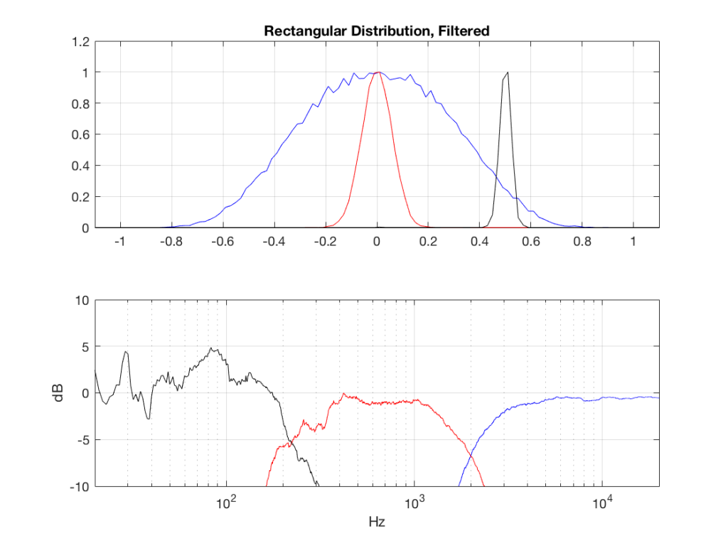
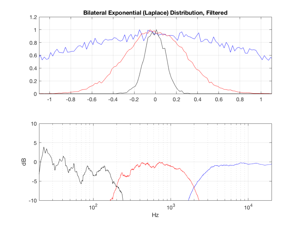
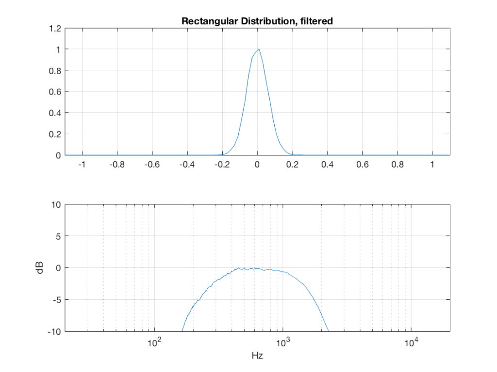
I made noise signals (length 2^16 samples, fs=2^16) with different PDFs, and filtered them as if I were building a three-way loudspeaker with a 4th order Linkwitz-Riley crossover (without including the compensation for the natural responses of the drivers). The crossover frequencies were 200 Hz and 2 kHz (which are just representative, arbitrary values).
So, the filter magnitude responses looked like Figure 1.
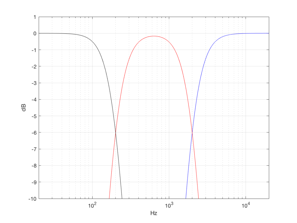
The resulting effects on the probability distribution functions are shown below. (Check the last posting for plots of the PDFs of the full-band signals – however note that I made new noise signals, so the magnitude responses won’t match directly.)
The magnitude responses shown in the plots below have been 1/3-octave smoothed – otherwise they look really noisy.
Post-script
This posting has a Part 1 that you’ll find here and a Part 2 that you’ll find here.
Probability Density Functions, Part 2
In a previous posting, I showed some plots that displayed the probability density functions (or PDF) of a number of commercial audio recordings. (If you are new to the concept of a probability density function, then you might want to at least have a look at that posting before reading further…)
I’ve been doing a little more work on this subject, with some possible implications on how to interpret those plots. Or, perhaps more specifically, with some possible implications on possible conclusions to be drawn from those plots.
Full-band examples
To start, let’s create some noise with a desired PDF, without imposing any frequency limitations on the signal.
To do this, I’ve ported equations from “Computer Music: Synthesis, Composition, and Performance” by Charles Dodge and Thomas A. Jerse, Schirmer Books, New York (1985) to Matlab. That code is shown below in italics, in case you might want to use it. (No promises are made regarding the code quality… However, I will say that I’ve written the code to be easily understandable, rather than efficient – so don’t make fun of me.) I’ve made the length of the noise samples 2^16 because I like that number. (Actually, it’s for other reasons involving plotting the results of an FFT, and my own laziness regarding frequency scaling – but that’s my business.)
Uniform (aka Rectangular) Distribution
uniform = rand(2^16, 1);
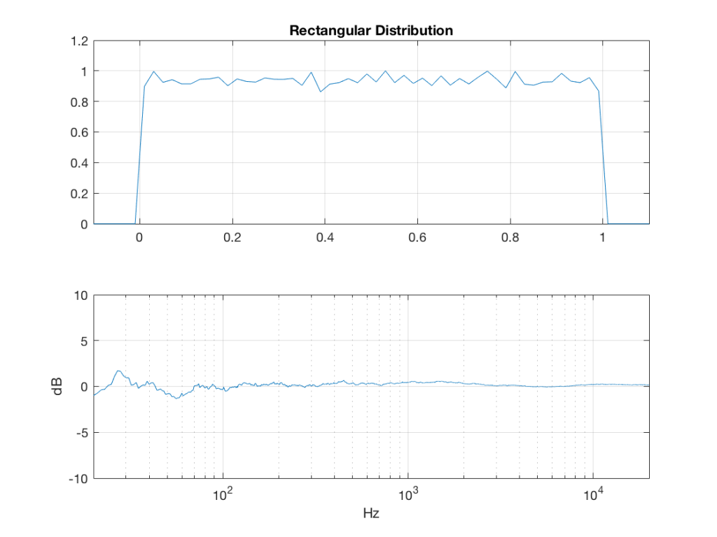
Of course, as you can see in the plots in Figure 1, the signal is not “perfectly” rectangular, nor is it “perfectly” flat. This is because it’s noise. If I ran exactly the same code again, the result would be different, but also neither perfectly rectangular nor flat. Of course, if I ran the code repeatedly, and averaged the results, the average would become “better” and “better”.
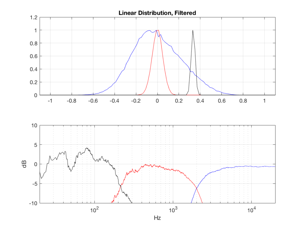
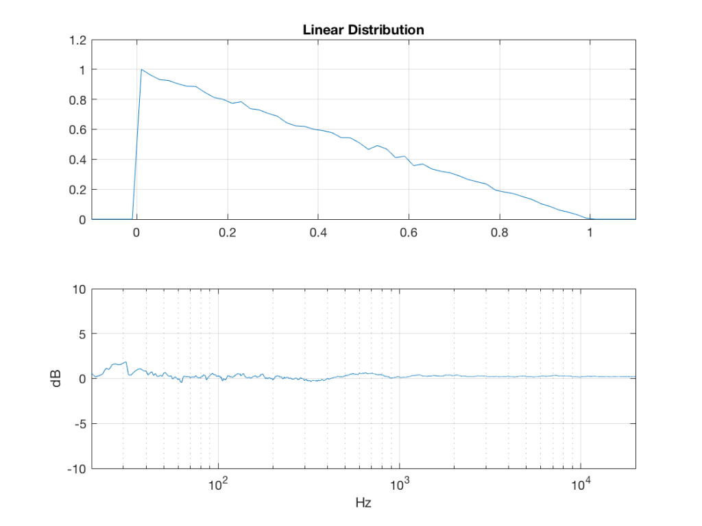
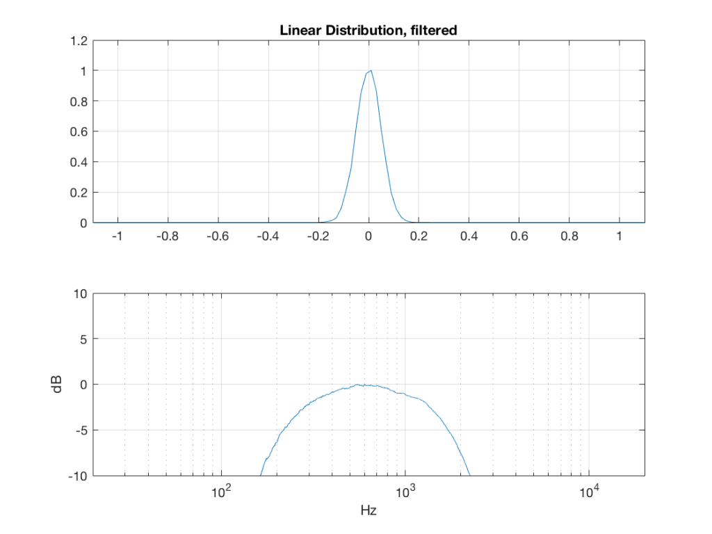
Linear Distribution
linear_temp_1 = rand(2^16, 1);
linear_temp_2 = rand(2^16, 1);
temp_indices = find(linear_temp_1 < linear_temp_2);
linear = linear_temp_2;
linear(temp_indices) = linear_temp_1(temp_indices);
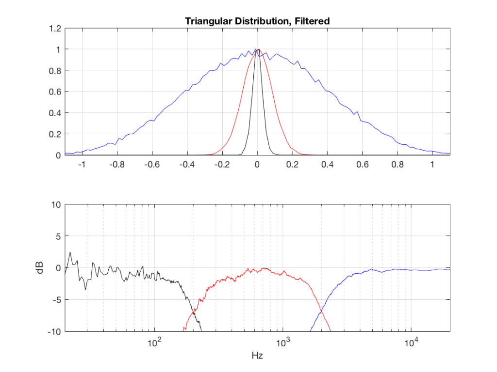
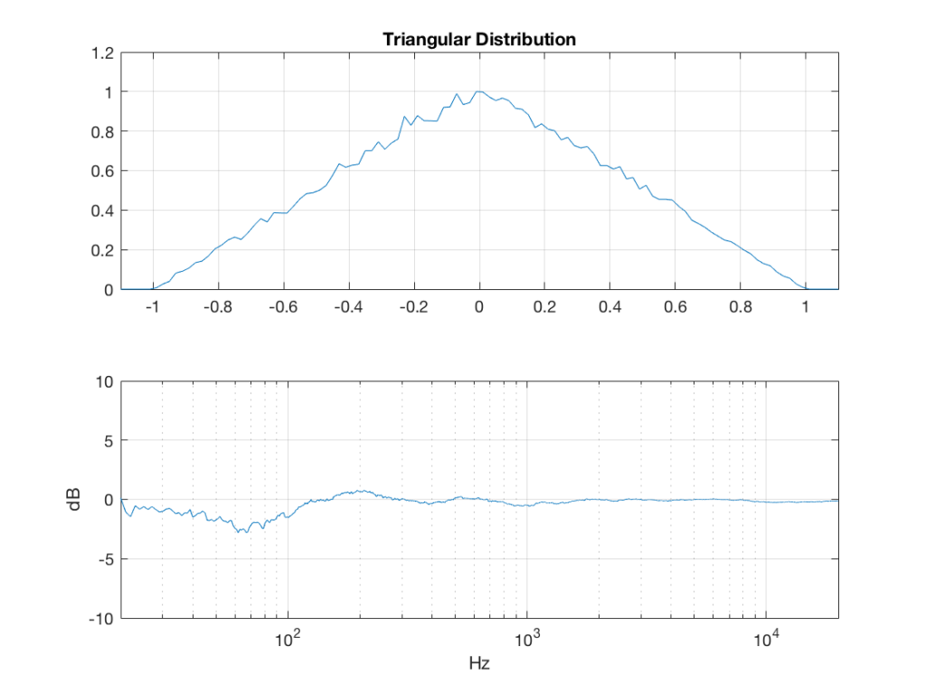
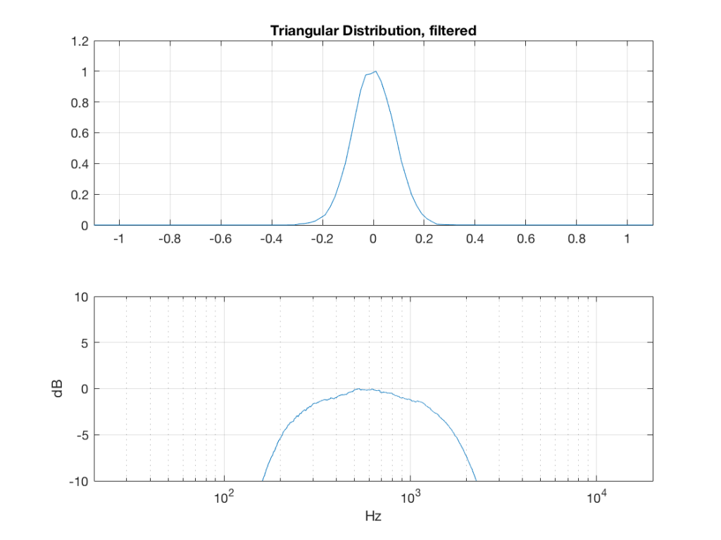
Triangular Distribution
triangular = rand(2^16, 1) – rand(2^16, 1);
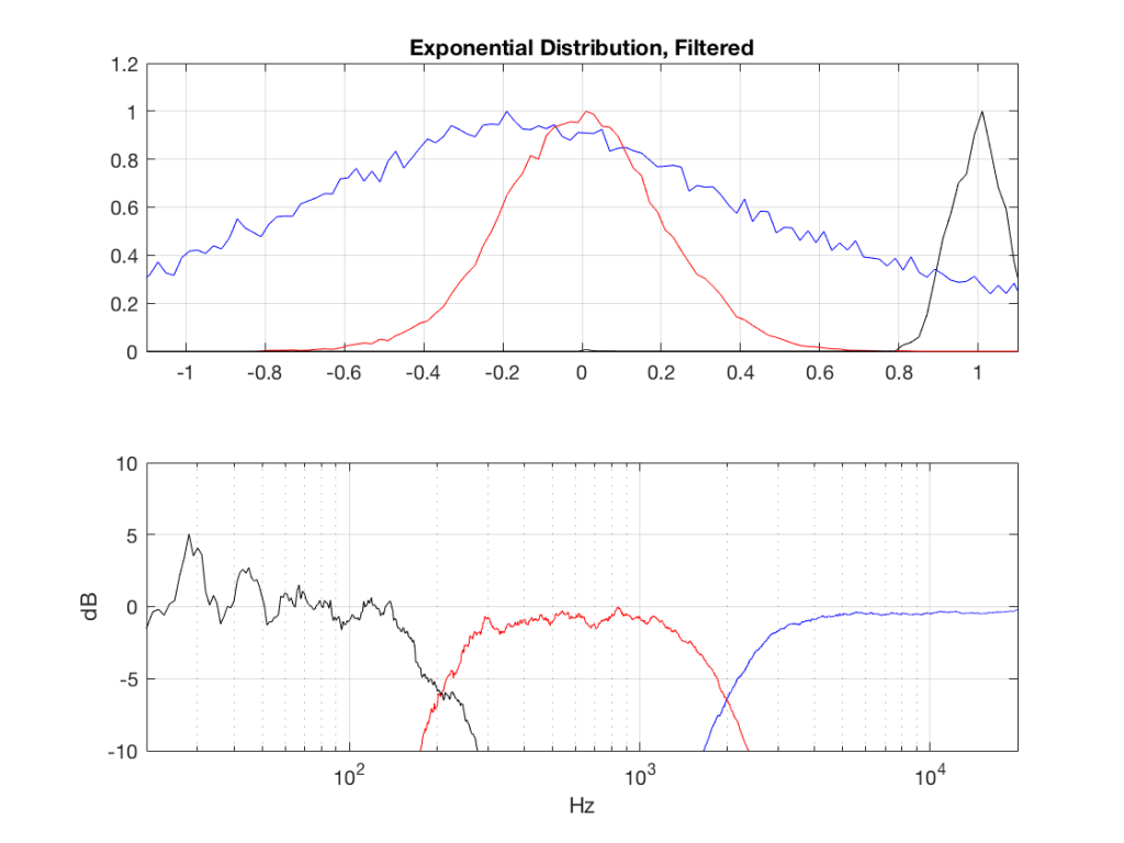
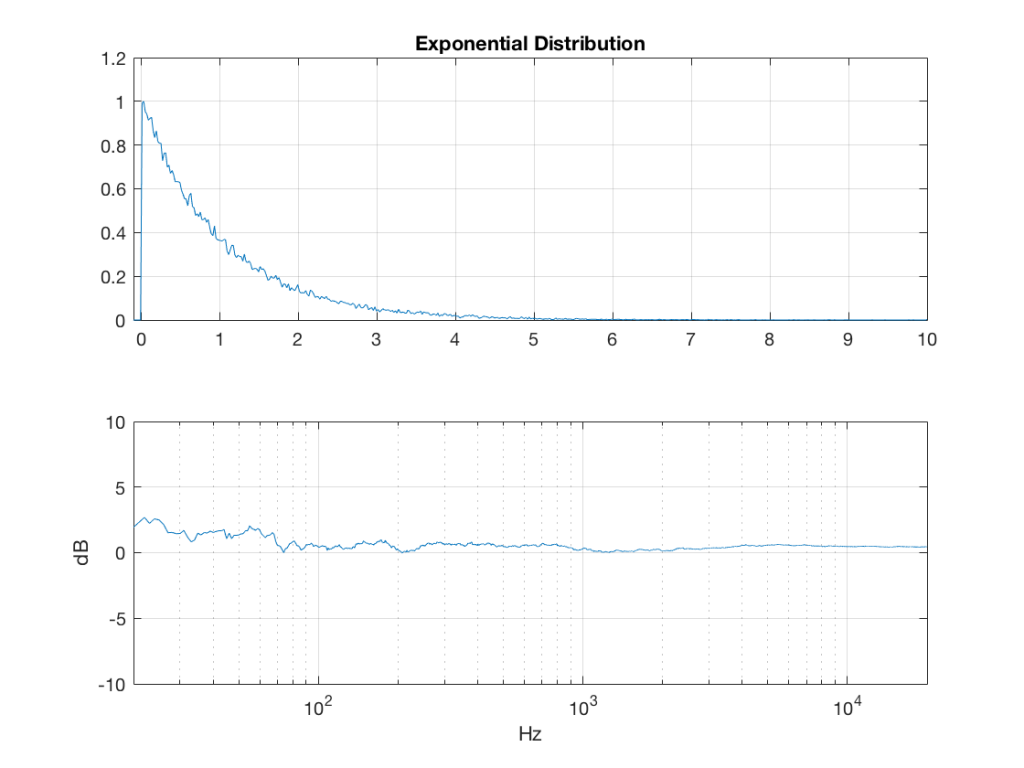
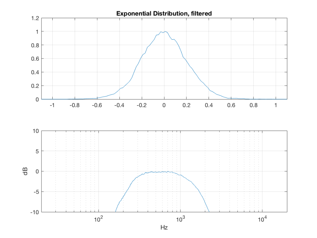
Exponential Distribution
lambda = 1; % lambda must be greater than 0
exponential_temp = rand(2^16, 1) / lambda;
if any(exponential_temp == 0) % ensure that no values of exponential_temp are 0
error(‘Please try again…’)
end
exponential = -log(exponential_temp);
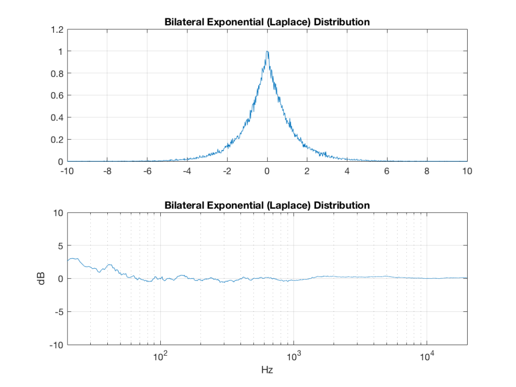
Bilateral Exponential Distribution (aka Laplacian)
lambda = 1; % must be greater than 0
bilex_temp = 2 * rand(2^16, 1);
% check that no values of bilex_temp are 0 or 2
if any(bilex_temp == 0)
error(‘Please try again…’)
end
bilex_lessthan1 = find(bilex_temp <= 1);
bilex(bilex_lessthan1, 1) = log(bilex_temp(bilex_lessthan1)) / lambda;
bilex_greaterthan1 = find(bilex_temp > 1);
bilex_temp(bilex_greaterthan1) = 2 – bilex_temp(bilex_greaterthan1);
bilex(bilex_greaterthan1, 1) = -log(bilex_temp(bilex_greaterthan1)) / lambda;
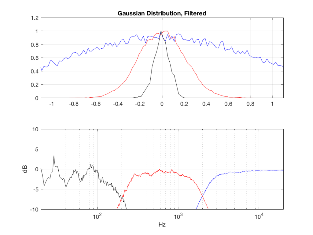
Gaussian
sigma = 1;
xmu = 0; % offset
n = 100; % number of random number vectors used to create final vector (more is better)
xnover = n/2;
sc = 1/sqrt(n/12);
total = sum(rand(2^16, n), 2);
gaussian = sigma * sc * (total – xnover) + xmu;
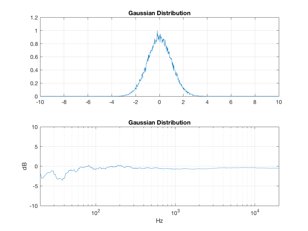
Of course, if you are using Matlab, there is an easier way to get a noise signal with a Gaussian PDF, and that is to use the randn() function.
The effects of band-passing the signals
What happens to the probability distribution of the signals if we band-limit them? For example, let’s take the signals that were plotted above, and put them through two sets of two second-order Butterworth filters in series, one set producing a high-pass filter at 200 Hz and the other resulting in a low-pass filter at 2 kHz .(This is the same as if we were making a mid-range signal in a 4th-order Linkwitz-Riley crossover, assuming that our midrange drivers had flat magnitude responses far beyond our crossover frequencies, and therefore required no correction in the crossover…)
What happens to our PDF’s as a result of the band limiting? Let’s see…
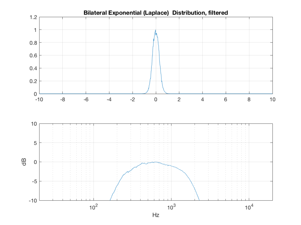
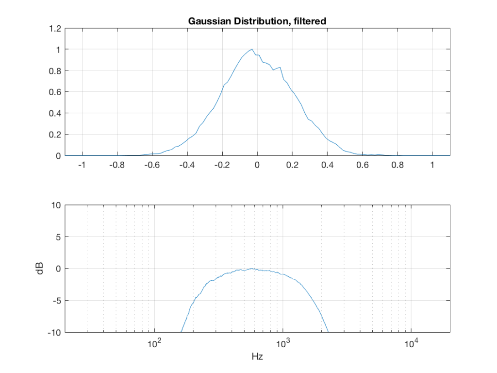
So, what we can see in Figures 7 through 12 (inclusive) is that, regardless of the original PDF of the signal, if you band-limit it, the result has a Gaussian distribution.
And yes, I tried other bandwidths and filter slopes. The result, generally speaking, is the same.
One part of this effect is a little obvious. The high-pass filter (in this case, at 200 Hz) removes the DC component, which makes all of the PDF’s symmetrical around the 0 line.
However, the “punch line” is that, regardless of the distribution of the signal coming into your system (and that can be quite different from song to song as I showed in this posting) the PDF of the signal after band-limiting (say, being sent to your loudspeaker drivers) will be Gaussian-ish.
And, before you ask, “what if you had only put in a high-pass or a low-pass filter?” – that answer is coming in a later posting…
Post-script
This posting has a Part 1 that you’ll find here, and a Part 3 that you’ll find here.