By now, we should know a couple of things:
- you cannot just stick a crossover in front of some loudspeaker drivers and expect the total system to behave
- the on-axis response and the power response of a loudspeaker are related to each other
- the power response is also very dependent on the directivity characteristics of the individual drivers and they way they interact (including the crossover’s effects) in three-dimensional space
- if you fix something for the on-axis response, you might do damage to the power response
Now we’re going to do something that I didn’t do in the previous posting. I’ll use the crossover responses as a TARGET for the total response of the crossover + driver outputs.
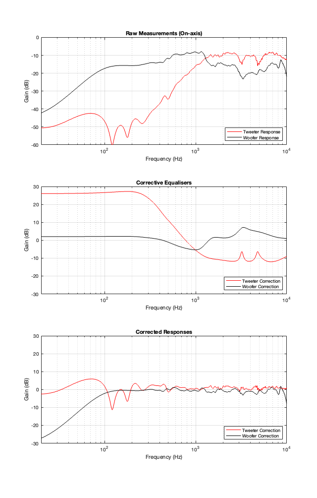
The top plot in Figure 11.1 shows the magnitude responses of the raw measurements of the tweeter and woofer that we looked at in Part 10. I then used these measurements to quickly make some agressive equalisation curves to force them to be flat-ish. These two equalisation filters are shown in the middle plot of Figure 11.1. Each of these is the product of a LOT of filters that I put in to result in the curves of the combined total responses that you see in the bottom of Figure 11.1.
In theory, if you play the tweeter and woofer through their respective equalisers, you will be able to measure the magnitude responses that you see there in the bottom of Figure 11.1. Of course, a 1″ tweeter can play a 20 Hz sine tone, it just can’t do it very loudly. So, this is NOT the solution to making a loudspeaker. This is just for illustrative purposes.
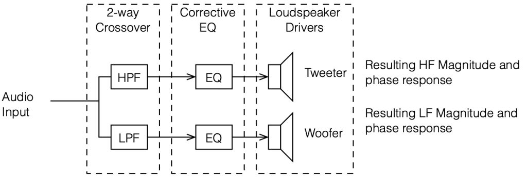
If I then apply our crossovers to these equalised loudspeaker drivers as shown in the signal flow above, I get the plots below.
4th order Linkwitz Riley
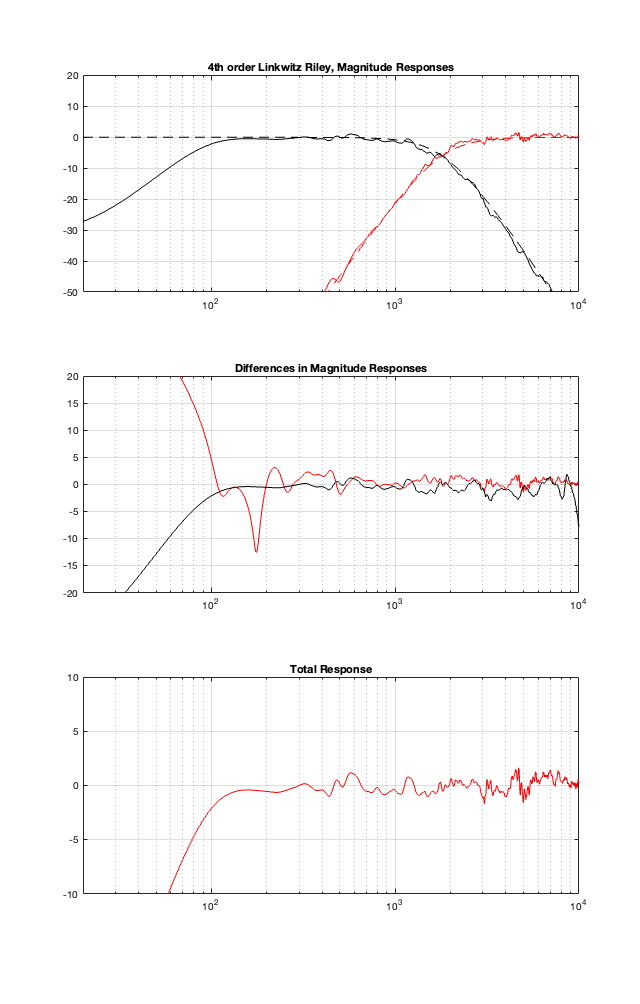
The top plot of Figure 11.3 shows the target magnitude responses of a 4th-order Linkwitz Riley crossover as the dotted lines. The solid lines show the measured outputs of the woofer and tweeter, including the corrective equalisation.
The middle plot shows the differences in what I want the crossover to do, and what the actual responses are at the outputs of the loudspeaker drivers. Again, in a perfect world, these would be two flat lines, sitting on 0 dB at all frequencies.
The bottom plot is the resulting on-axis response of the loudspeaker, combining the two outputs. Notice how much flatter it is than the one we had in Part 10. (the scale of this plot is much tighter than it was in the previous posting…)
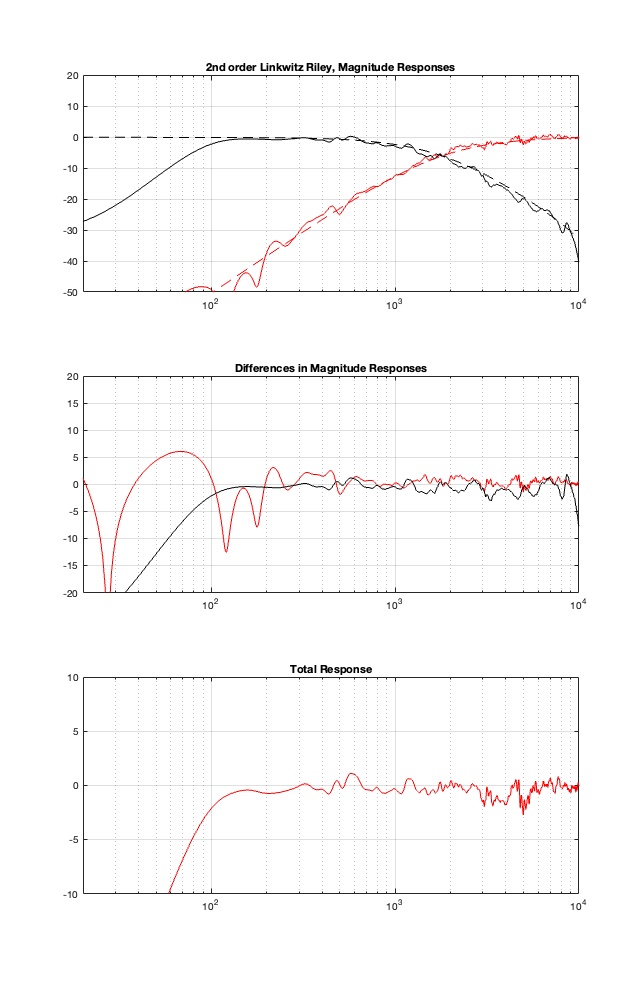
2nd Order Linkwitz Riley
2nd order Butterworth
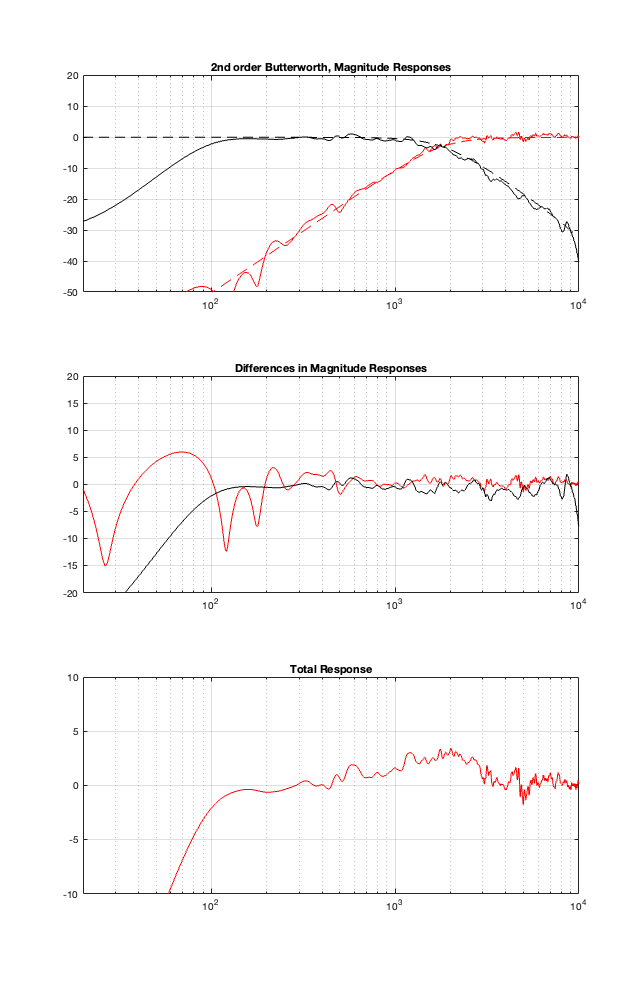
One comment here. Notice the +3 dB bump around the 1.8 kHz crossover, just like we would expect from a 2nd-order Butterworth crossover.
Constant Voltage
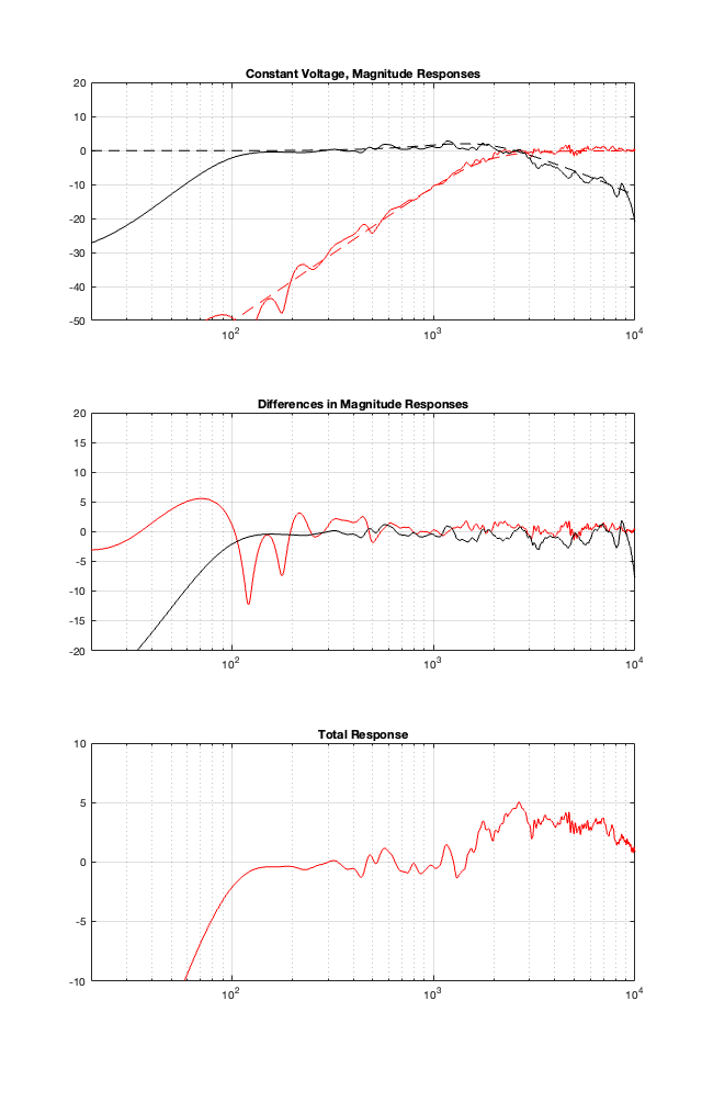
This one is interesting, but not surprising. You can see here that there is an unexpected high-shelving characteristic here in the total response. The reason for this is the combination of a number of things:
- the corrective EQ that I made was a bit quick-and-dirty, only using minimum phase filters
- a constant voltage crossover is very sensitive to phase variations in the two signal paths. If they don’t behave as one would expect (and they don’t in this loudspeaker because of my corrective EQ) then things get a little weird.
- Finally, take a look at the dotted lines. You can see there that the woofer has a lot of contribution in the high end. This combines with the previous point to make the total a little unpredictable.
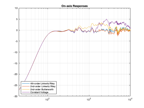
Just for comparison, here are the on-axis responses plotted in one figure.
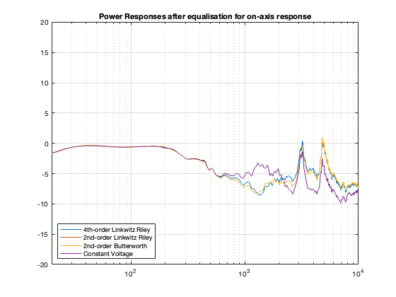
Power Responses
Finally, you might ask what the power responses look like for these loudspeakers. They’re shown below in Figure 11.8
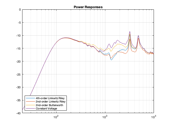
You might be surprised by the fact that, although most of our on-axis magnitude responses look pretty flat, the Power Responses are not nice, straight lines with a general downward slope. In fact, they have some pretty ugly peaks there. Why? This is because I did my equalisation based on only one on-axis measurement. So, by focusing all of my attention on that one point in space, I sacrificed the response of the spherical radiation. If we were making a loudspeaker for an anechoic chamber, and we had only one chair and no friends, this would be fine. However, this would NOT be a good solution for a loudspeaker that’s designed for a real room that has some reflections.
On the other hand, there is one interesting thing that’s worth noting in those plots.
The downward slope from about 150 Hz to about 1 kHz is the result of the woofer “beaming” as the frequency increases. The total power in the three-dimensional radiation of the loudspeaker drops because there’s less and less energy radiating backwards – and therefore less and less total power.
Above this, the power responses increase again because we’re moving into the tweeter, which is more omnidirectional in its low end.
Both of these points are another way of seeing the information shown in Figure 6 in this posting about loudspeaker directivity.
It’s also interesting to compare this plot to Figure 10.1 in Part 10. Notice that the transition in the slope just above 1 kHz has disappeared. This is because the responses of the two drivers have been cleaned up by the individual equalisation.
One last thing to notice is the that the similarity between the curves in this plot is a lot like the curves in Figure 10.3 in the previous posting. This is because, in both cases, I’m doing some kind of correction for the on-axis response. In Part 10, I put in a correction for the on-axis response of the entire loudspeaker after the tweeter and woofer outputs were summed. In this posting, I corrected for the individual loudspeakers’ on-axis responses before summing them. Although the two methods are different, the end results are similar to each other. Another way to think of this is that correcting for the on-axis response makes the power responses of the different crossover types more similar to each other.
Just for completeness, Figure 11.9 shows the Power Responses if I were to apply a “dumb” filter that REALLY flattens the on-axis response after all of this. You shouldn’t need to do this, since the individual drivers were flattened in advance. Compare this one to Figure 10.3 in Part 10.
N.B. About a week after I made this posting, I found an error in my Matlab code that calculated the plots. They’ve now been updated to the correct curves. The general conclusions listed in the text haven’t changed, but some of the little details have.
Extra note for the sake of transparency
Figure 11.9 was made using a method that is about as stupid and lazy as I could have possibly done. For each crossover type, all I did was to subtract the values shown in the plot in Figure 11.7 from those in Figure 11.8. This is probably not the way that you would implement a “flattening” filter in real life, but it is similar to the old-fashioned strategy used by systems that blindly make an FIR filter based on a single measurement.