Don’t trust everything you hear…

High-Resolution Audio: More is not necessarily better…

I’ve been collecting some so-called “high-resolution” audio files over the past year or two (not including my good ol’ SACD’s and DVD-Audio’s that I bought back around the turn of the century… Or my old 1/4″, half-track, 30 ips tapes that I have left over from the past century. (Please do not add a comment at the bottom about vinyl… I’m not in the mood for a fight today.) Now, let’s get things straight at the outset. “High Resolution” means many things to many people. Some people say that it means “sampling rates above 44.1 kHz”. Other people say that it means “sampling rates at 88.2 kHz or higher”. Some people will say that it means 24 bits instead of 16, and sampling rate arguments are for weenies. Other people say that if it’s more than one bit, it ain’t worth playing. And so on and so on. For the purposes of this posting, let’s say that “high resolution” is a blanket marketing term that is used by people these days when they’re selling an audio file that you can download that is has a bit rate that is higher than 44.1 kHz / 16 bits or 1378.125 kbps. (You can calculate this yourself as follows: 44100 samples per second * 16 bits per sample * 2 channels / 1024 bits in a kilobit = 1378.125) I’ll also go on record (ha ha…) as saying that I would rather listen to a good recording of a good tune played by good musicians recorded at 44.1 kHz / 16 bit (or even worse!) than a bad recording (whatever that means) of a boring tune performed poorly by musicians that are encumbered neither by talent nor the interest to rehearse (or any recording that used an auto-tuner). All of that being said, I will also say that I am skeptical when someone says that something is something when they could get away with it being nothing. So, I like to check once-and-a-while to see if I’m getting what I was sold. So, I thought I might take some of my legally-acquired LPCM “high-resolution audio” files and do a quick analysis of their spectral content, just to see what’s there. In order to do this, I wrote a little MATLAB script that

loads one channel of my audio file
takes a block of 2^18 samples multiplied by a Blackman-Harris function and does an 2^18-point FFT on it
moves ahead 2^18 samples and repeats the previous step over and over until it gets to the end of the recording (no overlapping… but this isn’t really important for what I’m doing here…)
looks through all of the FFT results and take the maximum value of all FFT results for each FFT bin (think of it as a peak monitor with an infinite hold function on each frequency bin)
I plot the final result

So, the graphs below are the result of that process for some different tunes that I selected from my collection.

Track #1

Track 1 (an 88.2/24 file) is plotted first. Not much to tell here. You can see that, starting at about 1 kHz or so, the amplitude of the signals starts falling off. This is not surprising. If it did not do that, then we would use white noise instead of pink noise to give us a rough representation of the spectrum of music. You may notice that the levels seem quite low – the maximum level on the plot being about -40 dB FS but keep in mind that this is (partly) because, at no point in the tune, was there a sine wave that had a higher level than that. It does not mean that the peak level in the tune was -40 dB FS.

The second plot of the same tune just shows the details in the top 2 octaves of the recording. Since this is a 88.2 kHz file, then this means we’re looking at the spectrum from 11025 Hz to 44100 Hz. I’ve plotted this spectrum on a linear frequency scale so that it’s easier to see some of the details in the top end. This isn’t so important for this tune, but it will come in handy below…

Track #2

The full-bandwidth plot for Track #2 (another 94/24 file) is shown below.

This one is interesting if you take a look up at the very high end of the plot – shown in detail in the figure below.

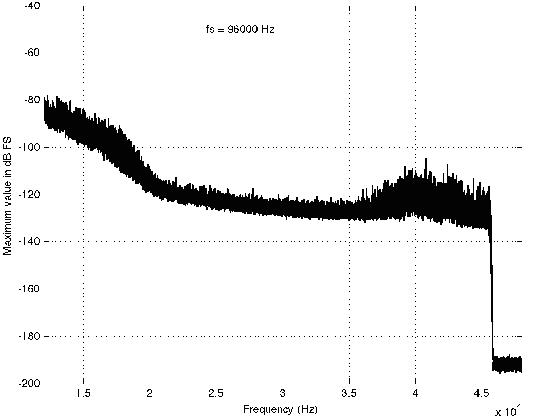
Here, you can see a couple of things. Firstly, you can see that there is a rise in the noise from about 35 kHz up to about 45 kHz. This is possibly (maybe even probably) the result of some kind of noise shaping applied to the signal, which is not necessarily a bad thing, unless you have equipment that has intermodulation distortion issues in the high end that would cause energy around that region to fold back down. However, since that stuff is at least 80 dB below maximum, I certainly won’t lose any sleep over it. Secondly, you can see that there is a very steep low pass filter (probably an anti-aliasing filter) that causes the signal to drop off above about 45 kHz. Note that the boost in the energy just before the steep roll-off might be the result of a peak in the low pass filter’s response – but I doubt it. It’s more a “maybe” than a “probably”. You may also have some questions about why the noise floor above about 46 kHz seems to flatten out at about -190 dB FS. This is probably not due to content in the recording itself. This is likely “spectral leakage” from the windowing that comes along with making an FFT. I’ll talk a little about this at the end of this article.

Track #3

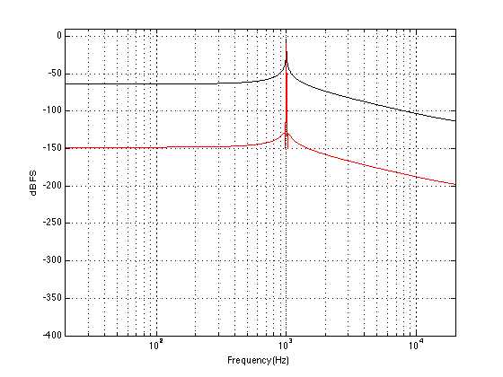
The third track on my hit list (another 94/24 file) is interesting…

Take a look at the spike there around 20 kHz… What the heck are they doing there!? Let’s take a look at the zoom (shown below) to see if it makes more sense.

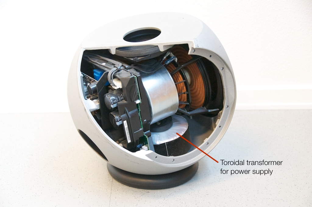
Okay, so zooming in more didn’t help – all we know is that there is something in this recording that is singing along at about 20 kHz at least for part of the recording (remember I’m plotting the highest value found for each FFT bin…). If you’re wondering what it might be, I asked a bunch of smart friends, and the best explanation we can come up with is that it’s noise from a switched-mode power supply that is somehow bleeding into the recording. HOW it’s bleeding into the recording is a potentially interesting question for recording engineers. One possibility is that one of the musicians was charging up a phone in the room where the microphones were – and the mic’s just picked up the noise. Another possibility is that the power supply noise is bleeding electrically into the recording chain – maybe it’s a computer power supply or the sound card and the manufacturer hasn’t thought about isolating this high frequency noise from the audio path. Or, maybe it’s something else.

Track #4

This last track is also sold as a 48 kHz, 24 bit recording. The total spectrum is shown below.

Track X: Full bandwidth — Track 4: Full bandwidth

This one is particularly interesting if we zoom in on the top end…

This one has an interesting change in slope as we near the top end. As you go up, you can see the knee of a low-pass filter around 20 kHz, and a second on around 23 kHz. This could be explained a couple of different ways, but one possible explanation is that it was originally a 44.1 kHz recording that was sample-rate converted to 48 kHz and sold as a higher-resolution file. The lower low-pass could be the anti-aliasing filter of the original 44.1 kHz recording. When the tune was converted to 48 kHz (assuming that it was…) there was some error (either noise or distortion) generated by the conversion process. This also had to be low-pass filtered by a second anti-aliasing filter for the new sampling rate. Of course, that’s just a guess – it might be the result of something totally different.

So what?

So what did I learn? Well, as you can see in the four examples above, just because a track is sold under the banner of “high-resolution”, it doesn’t necessarily mean that it’s better than a “normal resolution”recording. This could be because the higher resolution doesn’t actually give you more content or because it gives you content that you don’t necessarily want. Then again, it might mean that you get a nice, clean, recording that has the resolution you paid for, as in the first track. It seems that there is a bit of a gamble involved here, unfortunately. I guess that the phrase “don’t judge a book by its cover” could be updated to be “don’t judge a recording by its resolution” but it doesn’t really roll off the tongue quite so nicely, does it?

P.S.

Please do not bother asking what these four tracks are or where I bought them. I’m not telling. I’m not doing any of this to “out” anyone – I’m just saying “buyer beware”.

P.P.S

Please do not use this article as proof that high resolution recordings are a load of hooey that aren’t worth the money. That’s not what I’m trying to prove here. I’m just trying to prove that things are not always as they are advertised – but sometimes they are. Whether or not high res audio files are worth the money when they ARE the real McCoy is up to you.

Appendix

I mentioned some things above about “spectral leakage” and FFT windowing and a Blackman Harris function. Let’s do a quick run-through of what this stuff means without getting into too many details. When you do an FFT (a Fast Fourier Transform – but more correctly called a DFT or Discrete Fourier Transform in our case – but now I’m getting picky), you’re doing some math to convert a signal (like an audio recording) in the time domain into the frequency domain. For example, in the time domain, a sine wave will look like a wave, since it goes up and down in time. In the frequency domain, a sine wave will look like a single spike, because it contains only one frequency and no others. So, in a perfect world, an FFT would tell us what frequencies are contained in an audio recording. Luckily, it actually does this pretty well, but it has limitations. An FFT applied to an audio signal has a fixed number of outputs, each one corresponding to a certain frequency. The longer the FFT that you do, the more resolution you have on the frequencies (in other words, the “frequency bins” or “frequency centres” are closer together). If the signal that you were analysing only contained frequencies that were exactly the same as the frequency bins that the FFT was reporting on, then it would tell you exactly what was in the signal – limited only by the resolution of your calculator. However, if the signal contains frequencies that are different from the FFT’s frequency bins, then the energy in the signal “leaks” into the adjacent bins. This makes it look like there is a signal with a different frequency than actually exists – but it’s just a side effect of the FFT process – it’s not really there. The amount that the energy leaks into other frequency bins can be minimised by shaping the audio signal in time with a “windowing function”. There are many of these functions with different names and equations. I happened to use the Blackman Harris function because it gives a good rejection of spectral artefacts that are far from the frequency centre, and because it produces relatively similar artefact levels regardless of whether your signal is on or off the frequency bin of the FFT. For more info on this, read this.

Spectral leakage of Blackman-Harris windowing function. 1000 Hz, Fs=2^18, FFT Window length = 2^18 samples. The black plot shows the magnitude response calculated using an FFT and a rectangular windowing function. The red curve is with a Blackman Harris function. — Spectral leakage of Blackman-Harris windowing function. 1000 Hz at 0 dB FS, Fs=2^16, FFT Window length = 2^16 samples. The black plot shows the magnitude response calculated using an FFT and a rectangular windowing function. The red curve is with a Blackman Harris function. Note that the spectral leakage caused by the Blackman Harris function “bleeds” energy into all other bins, resulting in apparently much higher values than in the case of the rectangular windowing function.

This is a detail showing the peak of the response of for the 1000 Hz tone analysis. Note that the apparent level of the tone windowed using the Blackman Harris function is about 9 dB lower than when it’s windowed with a rectangular function.

Spectral leakage of Blackman-Harris windowing function. 1000.5 Hz, Fs=2^18, FFT Window length = 2^18 samples. The black plot shows the magnitude response calculated using an FFT and a rectangular windowing function. The red curve is with a Blackman Harris function. — Spectral leakage of Blackman-Harris windowing function. 1000.5 Hz at 0 dB FS, Fs=2^16, FFT Window length = 2^16 samples. The black plot shows the magnitude response calculated using an FFT and a rectangular windowing function. The red curve is with a Blackman Harris function. Now, since the frequency of the signal does not fall exactly on an FFT bin, the Blackman Harris – windowed signal appears “cleaner” than the one windowed using a rectangular function.

This is a detail showing the peak of the response of for the 1000.5 Hz tone analysis.

B&O Tech: BeoVision Avant Audio

#20 in a series of articles about the technology behind Bang & Olufsen loudspeakers

This was a presentation I did at a technical press event where we showed the BeoVision Avant for the first time. The video was done by one of the journalists at the event. The associated article (in Danish) is here at http://www.recordere.dk.

Solo for tree rings

B&O Tech: Free / Wall / Corner

#19 in a series of articles about the technology behind Bang & Olufsen loudspeakers

If you take a careful look around the connection panel of almost any Bang & Olufsen loudspeaker, you’ll find a three-position switch that is labelled something like “Free / Wall / Corner” or “F / W / C” or “Pos 1 / Pos 2 / Pos 3”. What does this do and how should you use it?

Part 1: Unreal acoustics

Let’s pretend that you have a loudspeaker that is perfectly omnidirectional, and it is in a free field (meaning that the sound that radiates from it is free to propagate forever without hitting anything – in other words, it’s floating in infinite space). Let’s then say that we measure the magnitude response of that loudspeaker and we find out that it has a perfectly flat response from 0 Hz to infinity Hz. Remember that the source is perfectly omnidirectional, so the response will be the same regardless of which direction you measure it from. This also means that if you do a lot of magnitude response measurements around the source and average them, it will also be flat, since the average of a whole bunch of the same thing is the same as any one of the things (i.e. the average of 5 & 5 & 5 & 5 & 5 & 5 & 5 is 5).

Fig 1. The average of the magnitude responses of a perfectly omnidirectional loudspeaker, measured at all points on a sphere around it.

Now let’s divide the infinite space in half with a very large, perfectly flat wall that extends infinitely – and we’ll put it fairly close to the loudspeaker. Now, if we do a magnitude response measurement at one position, we’ll see a response that is comprised of alternating boosts and cuts as we go up in frequency. This is caused by the interference between the direct sound of the loudspeaker and its reflection off the wall. These two sounds arrive at the measurement microphone at two different times – which means that different frequencies will be separated in phase differently. The higher the frequency, the greater the phase difference between the direct and reflected sounds. And, depending on the phase at any one frequency, the result may either be constructive interference (where the two signals add) or destructive interference (where they cancel each other). If it helps, an easier way to think of this is that the wall is a mirror that results in a reflection of the loudspeaker on the other side of it. The sound that arrives at the microphone is the combination of the two loudspeakers (the real one and the one on the other side of the mirror). If we do an averaged pressure response measurement, the averaging that we have to do results in the fact that we lose the phase information in each of our individual measurements. However, each individual response that we measure has peaks and dips that affects how it adds to the other responses. In the very low frequencies the “two” loudspeakers are very close together relative to the very long wavelengths of low frequencies in air – so they add together almost perfectly. This means that the total output will be doubled at the very low end – 200% of the output (or 6 dB more) than without the wall. At very high frequencies, the outputs of the two loudspeakers add randomly – sometimes increasing, sometimes cancelling the total. The end result of this average is a messy response, but is roughly the same level as 141% (or 3 dB more) than if the wall weren’t there. (Note that the low end is 2 times louder, (because there are two “sources” – the real one and the reflected one. However, the high end is 1.41 times louder. 1,41 is the square root of 2 – the reason for this involves an explanation of power being proportional to the square of the pressure, so doubling the power results in multiplying the pressure by sqrt(2).) Take a look at Figures 2 and 3. You’ll see that the result of placing the theoretical wall near the theoretical loudspeaker is that the low end and the high end are boosted – but the low end is boosted about 3 dB more than the high end. If you compare Figures 2 and 3, you’ll see that the closer the loudspeaker is to the wall, the higher the top frequency of the “low end”.

Fig 2. The average of the magnitude responses of a perfectly omnidirectional loudspeaker, 30 cm from an infinitely-extending flat wall, measured at all points on a half-sphere around it.

Fig 3. The average of the magnitude responses of a perfectly omnidirectional loudspeaker, 100 cm from an infinitely-extending flat wall, measured at all points on a half-sphere around it.

If you divide space once more, using a second wall that is perpendicular to the first (so now your speaker is on the floor, next to a wall, for example), you are doubling the number of “loudspeakers” again. Now we have one “real” loudspeaker and 3 reflections. Let’s forget about the magnitude response at one location for now and just deal with the power response, since that’s a little less complicated. Now we have 4 times the output (or 12 dB more) in the low frequencies and, 2 times the output (or 6 dB more) in the high frequency ranges. (Notice again that the multiplier for the output in the low end is the number of loudspeakers – either real or reflected – and that the multiplier for the output in the high frequencies is the square root of that number.)

Fig 4. The average of the magnitude responses of a perfectly omnidirectional loudspeaker, 30 cm from each of two, perpendicular infinitely-extending flat walls, measured at all points on a quarter-sphere around it.

Fig 5. The average of the magnitude responses of a perfectly omnidirectional loudspeaker, 100 cm from each of two, perpendicular infinitely-extending flat walls, measured at all points on a quarter-sphere around it.

Fig 6. The average of the magnitude responses of a perfectly omnidirectional loudspeaker, different distances from two perpendicular infinitely-extending flat walls (30 cm and 100 cm away), measured at all points on a quarter-sphere around it.

Finally, let’s add one last wall, perpendicular to the other two (i.e. two walls and the floor). This resuts in a total of 8 sources (one real and 7 reflected) which means that the output will be 8 times louder (or 18 dB) in the low end (than if the walls weren’t there) and 2.8 (sqrt(8)) times louder (or 9 dB) in the high end.

Fig 7. The average of the magnitude responses of a perfectly omnidirectional loudspeaker, 30 cm from each of three, perpendicular infinitely-extending flat walls, measured at all points on an eighth-sphere around it.

Fig 8. The average of the magnitude responses of a perfectly omnidirectional loudspeaker, 100 cm from each of three, perpendicular infinitely-extending flat walls, measured at all points on an eighth-sphere around it.

So, the first lesson to be learned here, for now, is that, in a theoretical world, where loudspeakers are perfectly omnidirectional and walls go forever, the more walls you have the bigger the bass boost. (Of course, you’ll also get a boost in the high end, but it will be smaller than the low-end boost, and you’ll probably compensate for that with the volume knob when the vocals and snare drum come in…) There is a second, nearly-as-important lesson. Look carefully, for example, at Figures 7 and 8. Starting in the low end, you can see the bass boost resulting from the collective reflections off the two walls. As you go up in frequency, you can see that the boost drops. However, before it levels out (albeit messily) at the high end, you can see that there is a deep drop in the level (i.e. in Figure 8, it’s at 100 Hz). This is because, for the particular wall distances we’re looking at, there is more cancellation of signals going on than there is constructive interference. So, the average is lower than if the walls weren’t there. This will be important later…

Part 2: Increasingly realistic acoustical behaviour

We can then take it one step further and consider that the very pretty graph shown in Figure 1 is extremely theoretical. A free field is an imaginary space – the reality is that a “free standing” loudspeaker is not really in a free field. For starters, it has to stand on something (unless you’re hanging it from the ceiling) – so the floor is not very far away – probably 1 m or so. Secondly, unless you live in a VERY large house, even when the loudspeaker is placed far from a wall, it’s probably not going to tens of metres away from any way. We can set a limit of something like 1 m on this – meaning, if you’re more than 1 m from any wall, we’ll call that “free”. This means that, in a real space, where the loudspeaker is at least 1 m from any surface, the response you get as a result of those three adjacent walls is roughly like the graph shown in Figure 8. The implications of this previous paragraph, in the real world, are important. What this means is that, when we do the sound design for a loudspeaker, we have to choose its position in a room rather carefully. Typically, it’s in a “free” position, which means, in a real world, about 1 m from each of the two adjacent walls (this isn’t measured exactly – everything in this article should be considered to be approximate). (Of course, loudspeakers that are, in all likelihood destined for a wall bracket are tuned on a wall instead.) So, the “free” position isn’t the same as the theoretical free field in Figure 1. It’s more like the not-very-close-to-a-surface case shown in Figure 8. The behaviour of the loudspeaker in this location is then the “reference” – the goal is then to ensure that, if a customer places the same loudspeaker against one wall or in a corner of two walls, the loudspeaker will sound the same as it does in the reference position. We do this by looking at the difference between the averaged response of the loudspeaker in the “wall” or “corner” location and the reference “free” position. For example, if we were making perfectly omnidirectional loudspeakers, and we say that 30 cm from a wall is close enough to call the loudspeaker in a “wall” position, then we would subtract the response curve shown in Figure 8 (the reference “Free” response) from the response shown in Figure 4. This difference, shown in Figure 9, below, is the “eq curve” applied to a loudspeaker that is placed closer to a wall. So, you can see that we get a large bump in the low end (in this case, with these dimensions) around 100 Hz, and dips below and above this peak (at 20 Hz and around 400 Hz).

The difference between Figure X and Figure X. — Fig 9. The difference between Figure 4 and Figure 8.

If we were making perfectly omnidirectional loudspeakers, and we compare a “corner” position 30 cm from three perpendicular wall, then we would subtract the response curve shown in Figure 8 (the reference “Free” response) from the response shown in Figure 7. This difference, shown in Figure 10, is the “eq curve” applied to a loudspeaker that is placed closer to a wall. So, you can see that we get a larger bump in the low end (in this case, with these dimensions), still around 100 Hz, and a dip above this peak (at around 300 Hz).

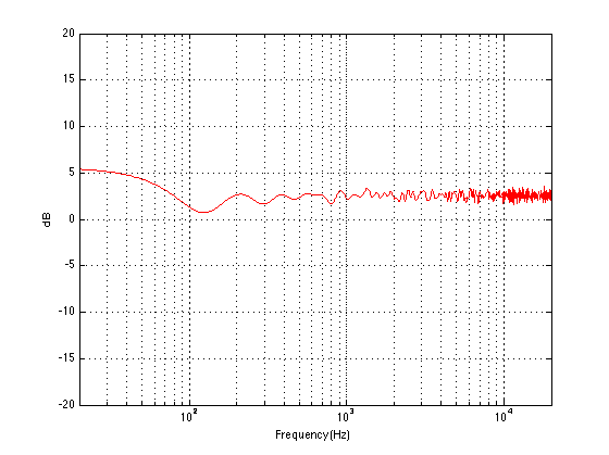
So, this means that, for these perfectly omnidirectional loudspeakers, considering only these dimensions, the equalisation filters we would have to apply to the loudspeaker to compensate for a “wall” or “corner” position would have to be the inverse of the curves in Figures 9 and 10. In other words, we would just flip them upside down to undo the change in the loudspeaker’s timbre as a result of its placement. However, in real life, loudspeakers are not omnidirectional at all frequencies. In real life, they don’t even have the same directional characteristics (omnidirectional or not…) as themselves at all frequencies. Due to their physical shape, the size of the loudspeaker drivers and the choice of crossover frequencies (amongst other things…) a typical loudspeaker will radiate different frequencies at different levels in different directions – even if it has been equalised to be perfectly flat on-axis in a free field. In addition, additional (perhaps unwanted) moving “parts” such as air flow in and out of a port, a slave driver or even a moving panel in the loudspeaker cabinet (see this article for a discussion about this) will not only affect the magnitude of a signal in a given direction, but also its phase relative to the on-axis response. So, what impact does reality have on the rule-of-thumb lessons learned above? Let’s take an only-slightly-more realistic example of a loudspeaker that is omnidirectional in the low frequency bands and very directional in the mid and upper frequency bands. Now, the energy in the low end will radiate forwards and backwards, reflecting off the wall (or walls) and still resulting in a boost. However, since the high frequency bands are not omnidirectional, you won’t get a boost from the reflections in the power response of the loudspeaker in the room. Consequently, the bass boost caused by the presence of the walls will be exaggerated due to the difference in directivity of the loudspeaker in different frequency bands. Of course, the actual directivity of a loudspeaker is considerably more complicated and messy than a simple description like “omni in the low end and beaming in the high end” – but we won’t delve very far into the details of that in this article. Let’s just stop at “real life is complicated”. The end result of this is that, if we do the same math as I used to do the plots shown above, but we include the actual directivity measurements of the actual loudspeaker, then we can calculate the final equalisation curves that we need to make the wall and corner positions sound more like the free position. An example of these curves are shown below in Figure 11. Note that these curves are applied to the “free” setting which, in the case of this loudspeaker, is the reference position in which it was tuned during the sound design process. The two things to note here are the dip at around 100 Hz which counteracts the boost that we see in the theoretical curves in Figures 9 and 10. There is also a slight boost around 200 Hz which compensates for the dip that can be seen in Figures 9 and 10. The very low end is untouched, since there is very little difference in the extreme low end of the loudspeaker. This is because, in a normal room, you can’t get far enough away for the walls to “not exist” at 20 Hz – the wavelength of the very low end is just too big.

19_actual_free_wall_corner_responses — Fig 11. The actual “Wall” and “Corner” filter curves for one of the BeoLab loudspeakers. Note that the “Free” setting is flat, since that is the room position in which the loudspeaker is tuned during the sound design process.

So, as you can see, the “Free / Wall / Corner” position switch, supplied on almost all Bang & Olufsen loudspeakers, is not merely a simple shelving filter with a 3 dB or 6 dB difference on the low end. It’s a rather complicated filter that is customised for each loudspeaker that we make, since it is dependent on the specific directional characteristics of that loudspeaker.