
Category: recordings
Immersive audio
Sony / EMI deal

Typical Errors in Digital Audio: Wrapping up
This “series” of postings was intended to describe some of the errors that I commonly see when I measure and evaluate digital audio systems. All of the examples I’ve shown are taken from measurements of commercially-available hardware and software – they’re not “beta” versions that are in development.
There are some reasons why I wrote this series that I’d like to make reasonably explicit.
- Many of the errors that I’ve described here are significant – but will, in some cases, not be detected by “typical” audio measurements such as frequency response or SNR measurements.
- For example, the small clicks caused by skip/insert artefacts will not show up in a SNR or a THD+N measurement due to the fact that the artefacts are so small with respect to the signal. This does not mean that they are not audible. Play a midrange sine tone (say, in the 2 -3 kHz region… nothing too annoying) and listen for clicks.
- As another example, the drifting time clock problems described here are not evident as jitter or sampling rate errors at the digital output of the device. These are caused by a clocking problems inside the signal path. So, a simple measurement of the digital output carrier will not, in any way, reveal the significance of the problem inside the system.
- Aliasing artefacts (described here) may not show up in a THD measurement (since aliasing artefacts are not Harmonic). They will show up as part of the Noise in a THD+N measurement, but they certainly do not sound like noise, since they are weirdly correlated with the signal. Therefore you cannot sweep them under the rug as “noise”…
- Some of the problems with some systems only exist with some combinations of file format / sampling rate / bit depth, as I showed here. So, for example, if you read a test of a streaming system that says “I checked the device/system using a 44.1 kHz, 16-bit WAV file, and found that its output is bit-perfect” Then this is probably true. However, there is no guarantee whatsoever that this “bit-perfect-ness” will hold for all other sampling rates, bit depths, and file formats.
- Sometimes, if you test a system, it will behave for a while, and then not behave. As we saw in Figure 10 of this posting, the first skip-insert error happened exactly 10 seconds after the file started playing. So, if you do a quick sweep that only lasts for 9.5 seconds you’ll think that this system is “bit-perfect” – which is true most of the time – but not all of the time…
- Sometimes, you just don’t get what you’ve paid for – although that’s not necessarily the fault of the company you’re paying…
Unfortunately, the only thing that I have concluded after having done lots of measurements of lots of systems is that, unless you do a full set of measurements on a given system, you don’t really know how it behaves. And, it might not behave the same tomorrow because something in the chain might have had a software update overnight.
However, there are two more thing that I’d like to point out (which I’ve already mentioned in one of the postings).
Firstly, just because a system has a digital input (or source, say, a file) and a digital output does not guarantee that it’s perfect. These days the weakest links in a digital audio signal path are typically in the signal processing software or the clocking of the devices in the audio chain.
Secondly, if you do have a digital audio system or device, and something sounds weird, there’s probably no need to look for the most complicated solution to the problem. Typically, the problem is in a poor implementation of an algorithm somewhere in the system. In other words, there’s no point in arguing over whether your DAC has a 120 dB or a 123 dB SNR if you have a sampling rate converter upstream that is generating aliasing at -60 dB… Don’t spend money “upgrading” your mains cables if your real problem is that audio samples are being left out every half second because your source and your receiver can’t agree on how fast their clocks should run.
So, the bad news is that trying to keep track of all of this is complicated at best. More likely impossible.
On the other hand, if you do have a system that you’re happy with, it’s best to not read anything I wrote and just keep listening to your music…
Typical Errors in Digital Audio: Part 8 – The Weakest Link
As a setup for this posting, I have to start with some background information…
Back when I was doing my bachelor’s of music degree, I used to make some pocket money playing background music for things like wedding receptions. One of the good things about playing such a gig was that, for the most part, no one is listening to you… You’re just filling in as part of the background noise. So, as the evening went on, and I grew more and more tired, I would change to simpler and simpler arrangements of the tunes. Leaving some notes out meant I didn’t have to think as quickly, and, since no one was really listening, I could get away with it.
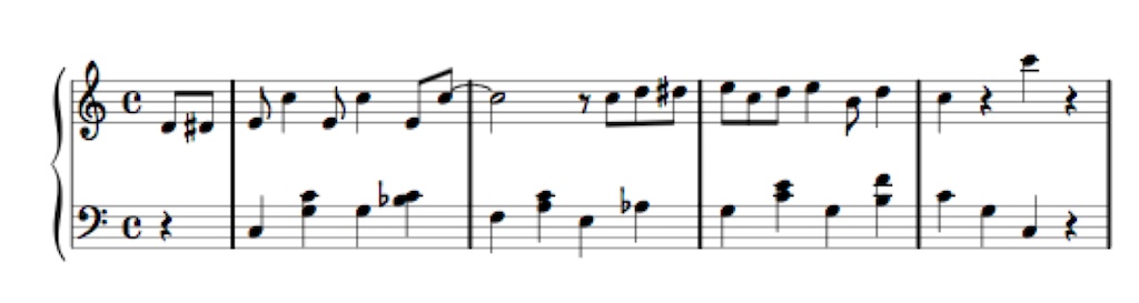
If you watch the short video above, you’ll hear the same composition played 3 times (the 4th is just a copy of the first, for comparison). The first arrangement contains a total of 71 notes, as shown below.

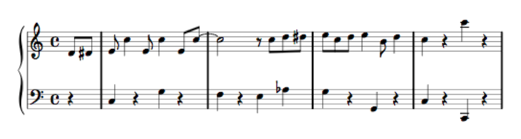
The second arrangement uses only 38 notes, as you can see in Figure 2, below.
The third arrangement uses even fewer notes – a total of only 27 notes, shown in Figure 3, below.
The point of this story is that, in all three arrangements, the piece of music is easily recognisable. And, if it’s late in the night and you’ve had too much to drink at the wedding reception, I’d probably get away with not playing the full arrangement without you even noticing the difference…
A psychoacoustic CODEC (Compression DECompression) algorithm works in a very similar way. I’ll explain…
If you do an “audiometry test”, you’ll be put in a very, very quiet room and given a pair of headphones and a button. in an adjacent room is a person who sees a light when you press the button and controls a tone generator. You’ll be told that you’ll hear a tone in one ear from the headphones, and when you do, you should push the button. When you do this, the tone will get quieter, and you’ll push the button again. This will happen over and over until you can’t hear the tone. This is repeated in your two ears at different frequencies (and, of course, the whole thing is randomised so that you can’t predict a response…)
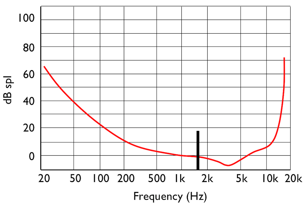
If you do this test, and if you have textbook-quality hearing, then you’ll find out that your threshold of hearing is different at different frequencies. In fact, a plot of the quietest tones you can hear at different frequencies it will look something like that shown in Figure 4.
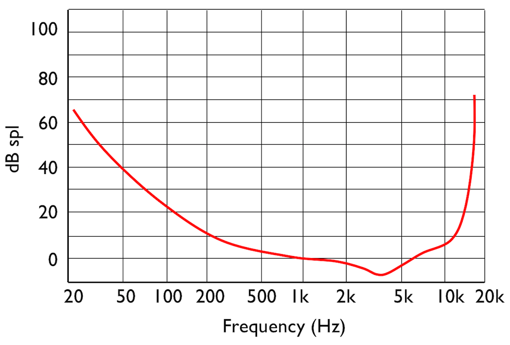
This red curve shows a typical curve for a threshold of hearing. Any frequency that was played at a level that would be below this red curve would not be audible. Note that the threshold is very different at different frequencies.

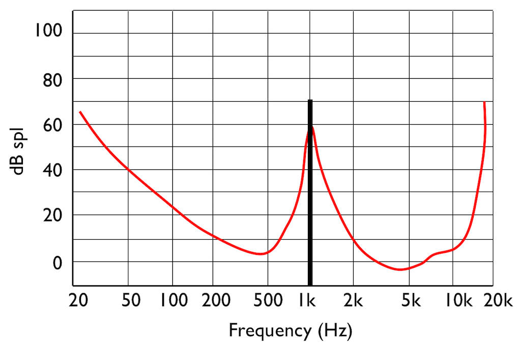
Interestingly, if you do play this tone shown in Figure 5, then your threshold of hearing will change, as is shown in Figure 6.
IF you were not playing that loud 1 kHz tone, and, instead, you played a quieter tone just below 2 kHz, it would also be audible, since it’s also above the threshold of hearing (shown in Figure 7.
However, if you play those two tones simultaneously, what happens?
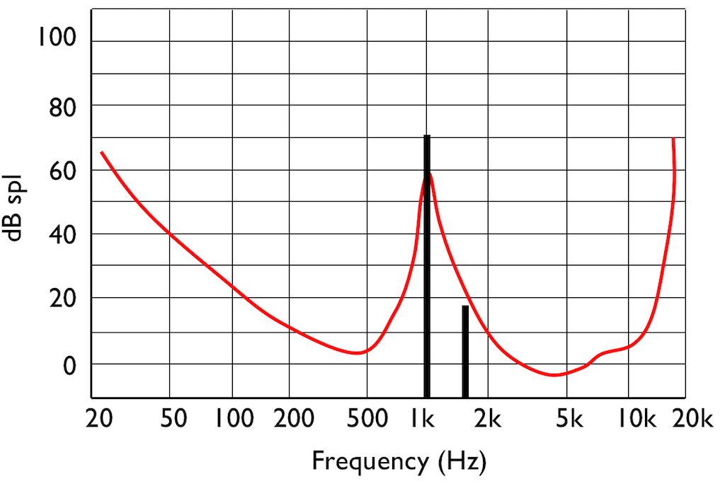
This effect is called “psychoacoustic masking” – the quieter tone is masked by the louder tone if the two area reasonably close together in frequency. This is essentially the same reason that you can’t hear someone whispering to you at an AC/DC concert… Normal people call it being “drowned out” by the guitar solo. Scientists will call it “psychoacoustic masking”.
Let’s pull these two stories together… The reason I started leaving notes out when I was playing background music was that my processing power was getting limited (because I was getting tired) and the people listening weren’t able to tell the difference. This is how I got away with it. Of course, if you were listening, you would have noticed – but that’s just a chance I had to take.
If you want to record, store, or transmit an audio signal and you don’t have enough processing power, storage area, or bandwidth, you need to leave stuff out. There are lots of strategies for doing this – but one of them is to get a computer to analyse the frequency content of the signal and try to predict what components of the signal will be psychoacoustically masked and leave those components out. So, essentially, just like I was trying to predict which notes you wouldn’t miss, a computer is trying to predict what you won’t be able to hear…
This process is a general description of what is done in all the psychoacoustic CODECs like MP3, Ogg Vorbis, AC-3, AAC, SBC, and so on and so on. These are all called “lossy” CODECs because some components of the audio signal are lost in the encoding process. Of course, these CODECs have different perceived qualities because they all have different prediction algorithms, and some are better at predicting what you can’t hear than others. Also, depending on what bitrate is available, the algorithms may be more or less aggressive in making their decisions about your abilities.
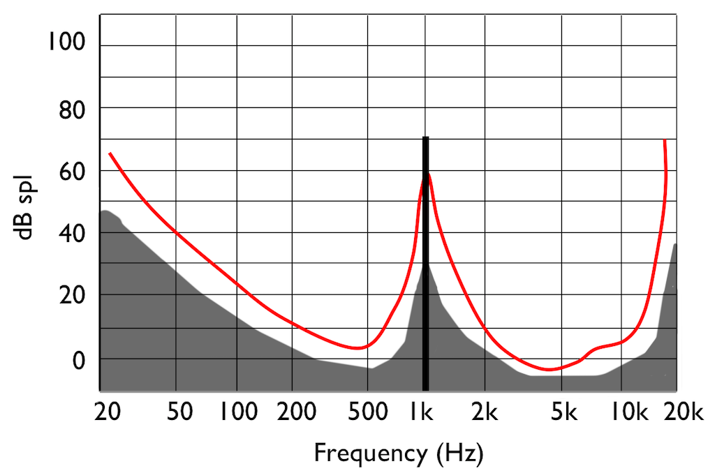
There’s just one small problem… If you remove some components of the audio signal, then you create an error, and the creation of that error generates noise. However, the algorithm has an trick up its sleeve. It knows the error it has created, it knows the frequency content of the signal that it’s keeping (and therefore it knows the resulting elevated masking threshold). So it uses that “knowledge” to shape the frequency spectrum of the error to sit under the resulting threshold of hearing, as shown by the gray area in Figure 9.
Let’s assume that this system works. (In fact, some of the algorithms work very well, if you consider how much data is being eliminated… There’s no need to be snobbish…)
Now to the real part of the story…
Okay – everything above was just the “setup” for this posting.
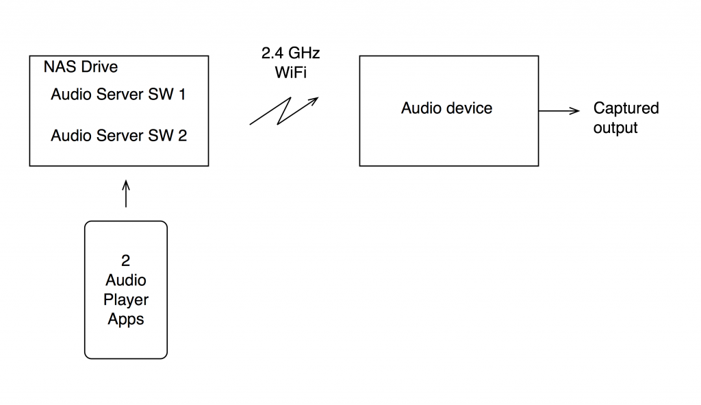
For this test, I put two .wav files on a NAS drive. Both files had a sampling rate of 48 kHz, one file was a 16-bit file and the other was a 24-bit file.
On the NAS drive, I have two different applications that act as audio servers. These two applications come from two different companies, and each one has an associated “player” app that I’ve put on my phone. However, the app on the phone is really just acting as a remote control in this case.
The two audio server applications on the NAS drive are able to stream via my 2.4 GHz WiFi to an audio device acting as a receiver. I captured the output from that receiver playing the two files using the two server applications. (therefore there were 4 tests run)
The content of the signal in the two .wav files was a swept sine tone, going from 20 Hz to 90% of Nyquist, at 0 dB FS. I captured the output of the audio device in Figure 10 and ran a spectrogram of the result, analysing the signal down to 100 dB below the signal’s level. The results are shown below.
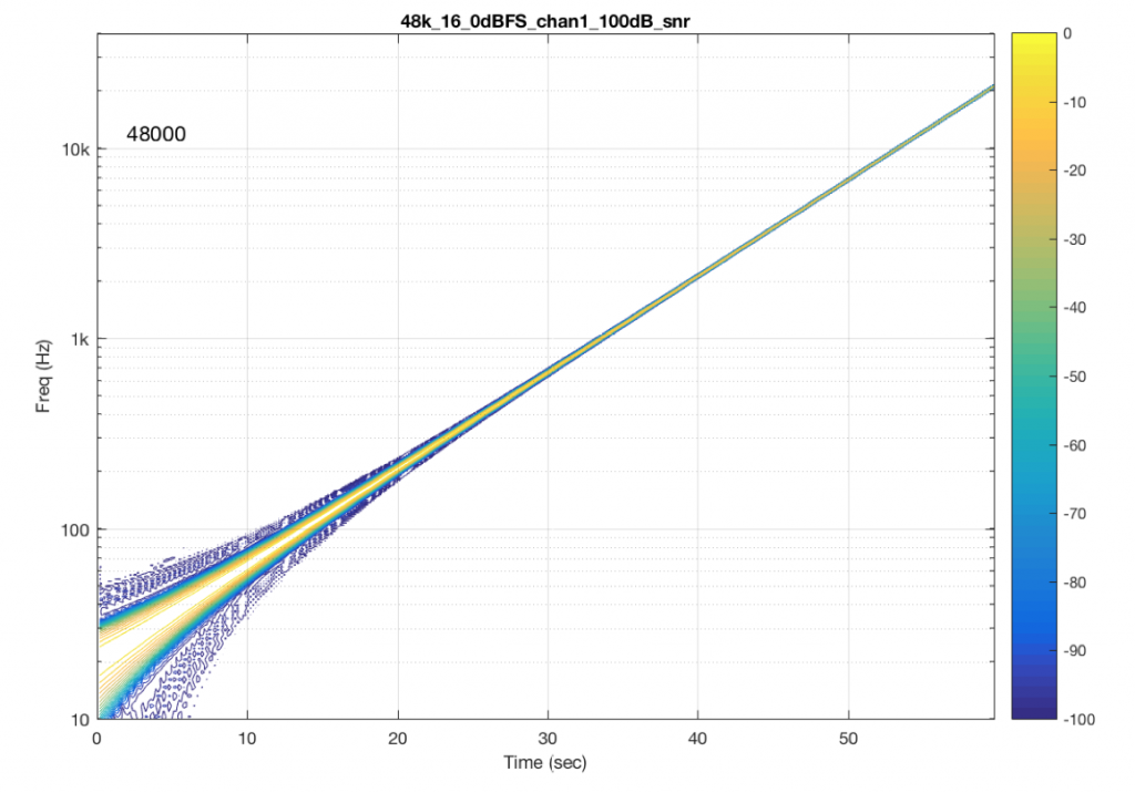


So, Figures 11 and 13 show the same file (the 16-bit version) played to the same output device over the same network, using two different audio server applications on my NAS drive.
Figures 12 and 14 also show the same file (the 24-bit version). As is immediately obvious, the “Audio Server SW 2” is not nearly as happy about playing the 24-bit file. There is harmonic distortion (the diagonal lines parallel with the signal), probably caused by clipping. This also generates aliasing, as we saw in a previous posting.
However, there is also a lot of visible noise around the signal – the “fuzzy blobs” that surround the signal. This has the same appearance as what you would see from the output of a psychoacoustic CODEC – it’s the noise that the encoder tries to “fit under” the signal, as shown in Figure 9… One give-away that this is probably the case is that the vertical width (the frequency spread) of that noise appears to be much wider when the signal is a low-frequency. This is because this plot has a logarithmic frequency scale, but a CODEC encoder “thinks” on a linear frequency scale. So, frequency bands of equal widths on a linear scale will appear to be wider in the low end on a log scale. (Another way to think of this is that there are as many “Hertz’s” from 0 Hz to 10 kHz as there are from 10 kHz to 20 kHz. The width of both of these bands is 10000 Hz. However, those of us who are still young enough to hear up there will only hear the second of these as the top octave – and there are lots of octaves in the first one. (I know, if we go all the way to 0 Hz, then there are an infinite number of octaves, but I don’t want to discuss Zeno today…))
Conclusion
So, it appears that “Audio Server SW 2” on my NAS drive doesn’t like sending 24 bits directly to my audio device. Instead, it probably decodes the wav file, and transcodes the lossless LPCM format into a lossy CODEC (clipping the signal in the process) and sends that instead. So, by playing a “high resolution” audio file using that application, I get poorer quality at the output.
As always, I’m not going to discuss whether this effect is audible or not. That’s irrelevant, since it’s dependent on too many other factors.
And, as always, I’m not going to put brand or model names on any of the software or hardware tested here. If, for no other reason, this is because this problem may have already been corrected in a firmware update that has come out since I tested it.
The take-home messages here are:
- an entire audio signal path can be brought down by one piece of software in the audio chain
- you can’t test a system with one audio file and assume that it will work for all other sampling rates, bit depths and formats
- Normally, when I run this test, I do it for all combinations of 6 sampling rates, 2 bit depths, and 2 formats (WAV and FLAC), at at least 2 different signal levels – meaning 48 tests per DUT
- What I often see is that a system that is “bit perfect” in one format / sampling rate / bit depth is not necessarily behaving in another, as I showed above..
So, if you read a test involving a particular NAS drive, or a particular Audio Server application, or a particular audio device using a file format with a sampling rate and a bit depth and the reviewer says “This system worked perfectly.” You cannot assume that your system will also work perfectly unless all aspects of your system are identical to the tested system. Changing one link in the chain (even upgrading the software version) can wreck everything…
This makes life confusing, unfortunately. However, it does mean that, if someone sounds wrong to you with your own system, there’s no need to chase down excruciating minutiae like how many nanoseconds of jitter you have at your DAC’s input, or whether the cat sleeping on your amplifier is absorbing enough cosmic rays. It could be because your high-res file is getting clipped, aliased, and converted to MP3 before sending to your speakers…
Addendum
Just in case you’re wondering, I tested these two systems above with all 6 standard sampling rates (44.1, 48, 88.2, 96, 176.4, and 192 kHz), 2 bit depths (16 & 24). I also did two formats (WAV and FLAC) and three signal levels (0, -1, and -60 dB FS) – although that doesn’t matter for this last comment.
“Audio Server SW 2” had the same behaviour in the case of all sampling rates – 16 bit files played without artefacts within 100 dB of the 0 dB FS signal, whereas 24-bit files in all sampling rates exhibited the same errors as are shown in Figure 14.
Typical Errors in Digital Audio: Part 7 – Just a sec…
We’ve seen in a previous posting that timing errors can occur in wireless audio systems. As we saw there, the wrong way to deal with this is to simply drop or repeat samples when the receiver realises it’s out of synchronisation with the transmitter. A better way to do it is to smoothly drift the sampling rate to either catch up or slow down – although this causes the modern-day equivalent of “wow and flutter”, since variations in the sampling rate will cause pitch shifts at the output. The trick here is to make changes slowly so as to get away with it…
However, what I didn’t address in that posting was how bad the problem can be – I only talked about how not to correct the problem when you know you have one.
So, let’s do a different (but related) test. I made a signal that consists of “digital black” – a long string of zeros – and therefore silence. Then, I made a single-sample spike every second (for example, every 44100 samples in a 44.1 kHz sampling rate system). In order to not make anything unhappy, I gave the clicks a value of 0.5 – so nothing is close to overloading…
Then, I transmitted that signal to an audio device wirelessly and recorded its output.
Figure 1, below, shows the original signal on top, and the recorded output of the device under test (the “DUT”) on the bottom.

You may notice that there is a little noise in the bottom plot. This is because this particular DUT has an acoustical output, and the noise you see there (partly) is acoustical noise in the room and measurement system.
Note that this plot shows only the first 5 seconds of a test that actually ran for 10 minutes.
Then, I wrote a little Matlab script that finds the spikes in each signal, and counts the number of samples between spikes. So, in a system running at 44.1 kHz I would expect that there is 1 spike every 44100 samples – both at the input to the system (the original signal) and its output. In other words, I’m finding out how far apart those spikes are with a resolution of 1 sample.
So, I find the duration between clicks at the output of the DUT, convert from samples to milliseconds, and plot the error over the full 600 seconds (10 minutes) of the test. In theory, there is no error – and each duration is exactly 1 second ±0 ms. In practice, however, this is not true.
For this posting, I tested two commercially-available devices, transmitting from the same device.
Figure 2 shows the results for that first device. As you can see there, one second at the device’s input does not correspond to 1 second at its output. It drifts from a little under 999.7 ms to a little over 1000.2 ms. Note that, for this test, I don’t know from the measurement how that change takes place – whether it’s shifting slowly or using a skip/insert strategy. I just know one version of how bad the problems is over time on a second-by-second basis.

Figure 3, below, shows the same analysis for another device. Notice that there are three colours in this plot, corresponding to three separate tests of the same device…

As you can see there, this device seems to be behaving most of the time, but occasionally gets a little lost and jumps by to about ±70 ms in a worst case. This means that, for this test, we can see that “1 second” can last anything between about 930 ms and 1070 ms. Note that this analysis doesn’t show what happens at the moment (or during the time) that jump occurs – we only know that it has happened sometime between clicks at the output.
You may be wondering why the plot in Figure 2 is more “jagged” than the one in Figure 3. This is mostly because the scale of the two plots is so different. If we were to zoom in to the plot in Figure 3, we would see that it is roughly as busy, as is shown below in Figure 4.

One significant difference between these two devices is that the first has an acoustical output and the second has an electrical output. This may cause you to wonder whether the acoustical noise in the first measurement contributes to the error. This may be possible. However, a 0.2 ms (or 200 µs) error is roughly equivalent to 9 samples at 44.1 kHz (or a 6.9 cm shift in distance between the DUT and the microphone). This is well outside the range of the error generated by acoustical noise – so that cannot be held responsible as being the only contributor to the error measurement.
I should say that the wireless audio protocol that was used for these two tests were the same… So, this is not a comparison of two different transmission systems. Also, as I mentioned above, the transmitter was the same for both DUT’s. So, the difference in results here are attributable to the skill and attention to the execution of the manufacturers of the two receiving devices.
As always, don’t bother asking which devices these DUT’s are. I’m not telling – primarily because it doesn’t matter. I’m just using these two devices as examples of errors I often see when I measure audio equipment…
One additional thing that might be of interest to geeks like me. That second DUT has a digital audio output, which is what I used to capture its signal. Interestingly, when I measure the sampling rate of that output with a digital audio signal analyser, the sampling rate is typically within 2 ppm of the correct frequency. So, ignoring the big spikes in Figure 3 (which are probably the result of buffer over- or under-runs) if the timing errors we see in Figure 4 were solely caused by a clock error that was visible on the digital audio output, then we should not see deviations of no more than approximately 2 microseconds per second. Instead, we see changes on the order of 1 to 2 milliseconds per second, which indicates a sample rate drift of 1000 to 2000 ppm… So, this means that, although the sampling rate of my transmitter and the output sampling rate of my receiver (the DUT) are nominally the same, AND there is very low jitter / error on the DUT’s output sampling rate, something else in the audio signal path is causing this error. In other words, a simple measurement of the digital output’s sampling rate is not adequate to verify that the DUT’s clock is behaving.
Save the past!

Typical Errors in Digital Audio: Part 5 – What time is it there?
I’m originally from Newfoundland – one of the few places in the world with a 1/2-hour time zone. So, when it’s 10:00 a.m. in Montreal, it’s 11:30 a.m. in St. John’s – my home town. This meant that, when I was a kid 40 years ago, and we would call our relatives in Toronto or Germany to wish them a Merry Christmas, there were two questions that you could always rely on being asked: (1) what’s the weather like there? and (2) what time is it there?
These days, I have a similar problem that is well-described by “Segal’s Law“. My iPhone and my wristwatch (an old analogue one with hands that go around pointing at the floor and the fridge…) are never synchronised… This is because of two things: (1) I probably did a bad job of setting my watch and (more importantly) (2) my watch runs just a little bit slowly…
So, let’s say, for example, that I set my watch to be EXACTLY in sync with my phone on a Monday morning at 9:00 a.m. As the week goes by, my iPhone and my watch drift apart, and, just for the sake of argument let’s say that, one week later, when my iPhone turns over to 9:00 a.m. on Monday morning, my wristwatch turns over to 8:59 a.m. So, I lose 1 minute per week on my watch.
(It’s pretty safe to assume that my iPhone is also not perfect – but it’s different because, every once in a while, it compares its internal clock with another, more accurate clock somewhere else via a connection across the Internet (which, we will assume, for the purposes of this discussion, works).)
Let’s consider this from a strange point of view. Let’s assume that
- I’m checking the time on my watch every minute, on the minute
- someone else is “fixing” my watch every week so that it’s correct at 9:00 a.m. on Mondays. They do this by adjusting the watch to the correct time 30 seconds before the iPhone says it’s 9:00 a.m.
- I don’t know that they’re doing this for me…
If we think about this from my perspective, I’ll live in a strange world where 8:59 on Mondays never exists. This is because at 8:58 and 30 seconds (on my watch), my friend re-sets the time to 8:59 and 30 seconds (while I’m not looking) to synchronise with the iPhone…
IF my watch was running fast – say, gaining one minute each week, then I would live in a different strange universe where 9:00 happens twice every Monday morning…
The basic problem here is that we have two clocks that do not run at the same rate – but they are expected to do so. So, we synchronise them regularly (in the above example, on Monday mornings at 9:00) – but between those synchronisation events, they drift apart in time.
So what?
The example above is very, very similar to the way a digital audio streaming system works – especially if you’re using a wireless connection between the transmitting device and a receiver.
Lets say that you’re playing a sound file that was recorded at 44.1 kHz and streaming it wirelessly to a receiver. I’m trying to be as generic as possible here, but I could be talking about a Bluetooth connection to a pair of headphones or a WiFi connection via DLNA to a device connected to a pair of loudspeakers, for example…
It is not unusual with such a connection for the transmitter to collect up a block of audio samples – say, 64 of them – and send them to the receiver’s input buffer. The receiver then pulls those samples out, one by one, and (eventually) sends them to a digital-to-analogue converter that produces a signal that (eventually) comes out as an audio signal. Then, 64/44100’ths of a second later (64 samples later) the transmitter sends another block, and so on and so on until the song ends.
This system works well if the clock inside the transmitter and the clock inside the receiver are perfectly synchronised. We can even be a little generous and say that they can drift apart a little – but not so much that we either run out of samples to play (because the receiver is playing them out faster than they’re coming in from the transmitter) or that we have samples left over to play when the next block comes in (because the receiver is playing them out slower than they’re coming in from the transmitter).
Dealing with this problem the right way
The right way to deal with this issue is for the receiver to always be checking what time it thinks it is when the block arrives from the transmitter. If the block arrives a little early, then the receiver should think “hmmmm, my clock is going too slowly – I’ll speed it up a bit”. If the block arrives a little late, then the receiver should adjust its clock to go a little slower.
So, in this case, the receiver has a basic, nominal speed for its internal clock – but it’s constantly adjusting it to be faster and slower to try and match the clock of the transmitter – but it can only do this adjustment at the block rate – the frequency at which the blocks of samples arrive, which is dependent on the block length (how many samples are in each block) and the sampling rate (how many samples per second). (Of course, this can result in “jitter and wander” problems if you’re not careful (I won’t talk about this here…) – so you have to pay a little attention to how quickly you’re adjusting your clock rate… but that’s “just” a matter of correct implementation.)
Dealing with this problem the wrong way
There is another way to deal with this problem, which, unfortunately, has measurable and possibly audible consequences. This implementation is basically the same as my original example, where I had a friend “fixing” my wristwatch once a week. You have a transmitter that sends blocks of samples to the receiver – and although these two devices should have exactly the same clock rate, they don’t.
Let’s say, for example, that the receiver is playing the samples faster than they’re being sent by the transmitter. This means that the two will slowly drift farther and farther apart until, eventually, the receiver will have to play a sample, but nothing has come in from the transmitter yet, so there’s no sample there to play. In this case, the receiver says “no problem, I’ll just play the last sample again, and the next block will come in while I’m doing that” – so it inserts an extra sample that is just a duplicate of the previous one.
If the receiver’s clock is going slower than the transmitter’s, then, as the two drift farther apart, we will get to a moment where the receiver will receive a new block of samples but it’s not done playing all of the samples in the previous block yet. In this event, it says “no problem, I’ll just leave that last sample out and move on to the next block to catch up” – so it skips a sample.
This is called a “Skip / Insert” strategy for dealing with clock synchronisation. It’s done by software and hardware engineers because it’s simple to implement, and, in many cases, a manufacturer can get away with this, since it is rarely audible for a couple of reasons.
Can this be measured?
The simple answer to this is “yes” – and it can be measured in a number of different ways. I’ll show one way below…
Can I hear it?
The honest answer to this question is “sometimes” – but it’s not as easy to detect as one might think. Of course, a skip/insert event (a duplicated sample or a dropped one) creates an artefact. However, the magnitude of this artefact relative to the “correct” signal is dependent on when it happens.
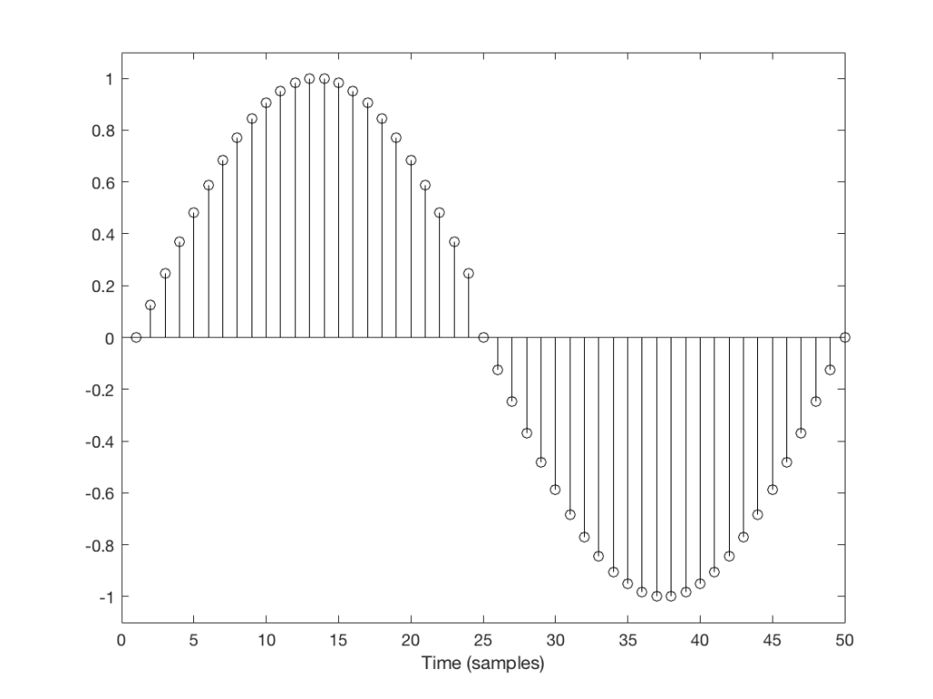
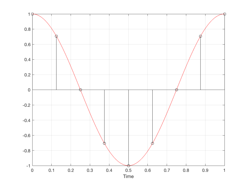
Let’s take a look at a couple of simple cases. We’ll “transmit” one period of a sine wave that should come out on the other side of the system looking like Figure 1.
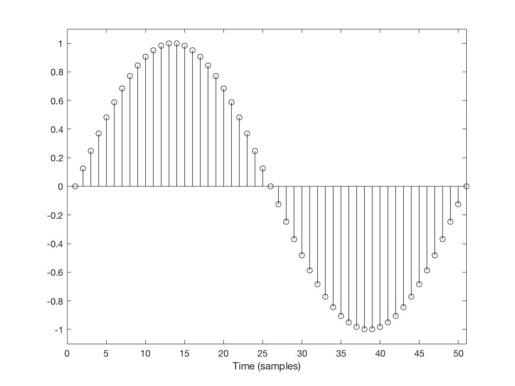
But what happens if we don’t get a block in time to keep outputting a signal? We insert a duplicate sample and hope that the block comes in before I have to send out another one. Examples of this are shown in Figures 2 and 3, below.

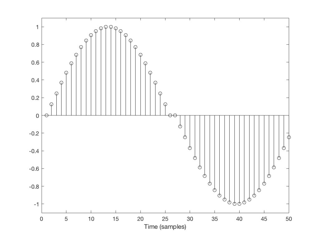
You’ll probably notice that it’s much easier to see which sample I duplicated in Figure 3 than in Figure 2. In Figure 3 it was sample number 26 that was duplicated. In Figure 2 it’s sample number 13.
The reason it’s easier to see the error in Figure 3 is that duplicating the sample causes an obvious change in the slope of the signal, whereas in Figure 2 it does not – the slope of the signal is 0, and by duplicating a sample, I am also making it 0 – but for a slightly longer time.
This does not mean that we did not generate an error. It just means that we’ll probably “get away with it” in the case of Figure 2, and we probably won’t in the case of Figure 3.
However, since the drifting of the two clocks (in the receiver and transmitter) are not dependent on the signal, there’s no way to know when this is going to happen.
And, of course, if this happens in the middle of a snare drum hit or a ssssinger sssstarting a word in a ssssong with the letter “s” – then we also won’t hear it because there’s so much going on (frequency-wise) that the artefact will be buried in the mess.
Also, since this clock drifting is usually not completely regular, the errors do not usually come in at a regular rate (although I’ve seen exceptions…). So, it’s not like you can listen for “a click every second” or “one per minute”. They happen when they happen – hopefully when you’re not listening and/or when the tune is busy enough to hide it.
A skip event is similar to an insert, as you can see in the two examples in Figures 4 and 5.
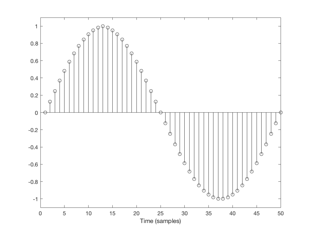
Again, I’ve intentionally put in these two skips in places where they are least obvious (Figure 4) and most obvious (Figure 5).
The real world
One of the tests that can be done on an audio system is to send a sinusoidal signal with a swept frequency through a system, capture the output, and then do a spectrogram of the result. In theory, if you see anything other than a single frequency at any one time at the output, then you know that something has happened to the signal. You would probably then need to go back and look at the output signal itself to start evaluating exactly what happened… This is a test that is used to evaluate one aspect of the performance of different sampling rate converters, for example, at this site.
Let’s take a sine sweep and run it through a system. The sweep goes up logarithmically in frequency from 20 Hz to about 90% of Nyquist (which would correspond to 20,000 Hz in a system running at 44.1 kHz) over 60 seconds and has a level of -1 dB FS. We’ll then capture the output in a system that is behaving perfectly and do a spectrogram of this, looking for artefacts down to some level below the signal level. (If you’re really geeky, you’ll know that this signal-to-error ratio is dependent on the window length of the FFT I’m using to create the spectrogram – but this is beyond our discussion today…).
An example of the output of a system that is behaving well is shown in Figure 6.
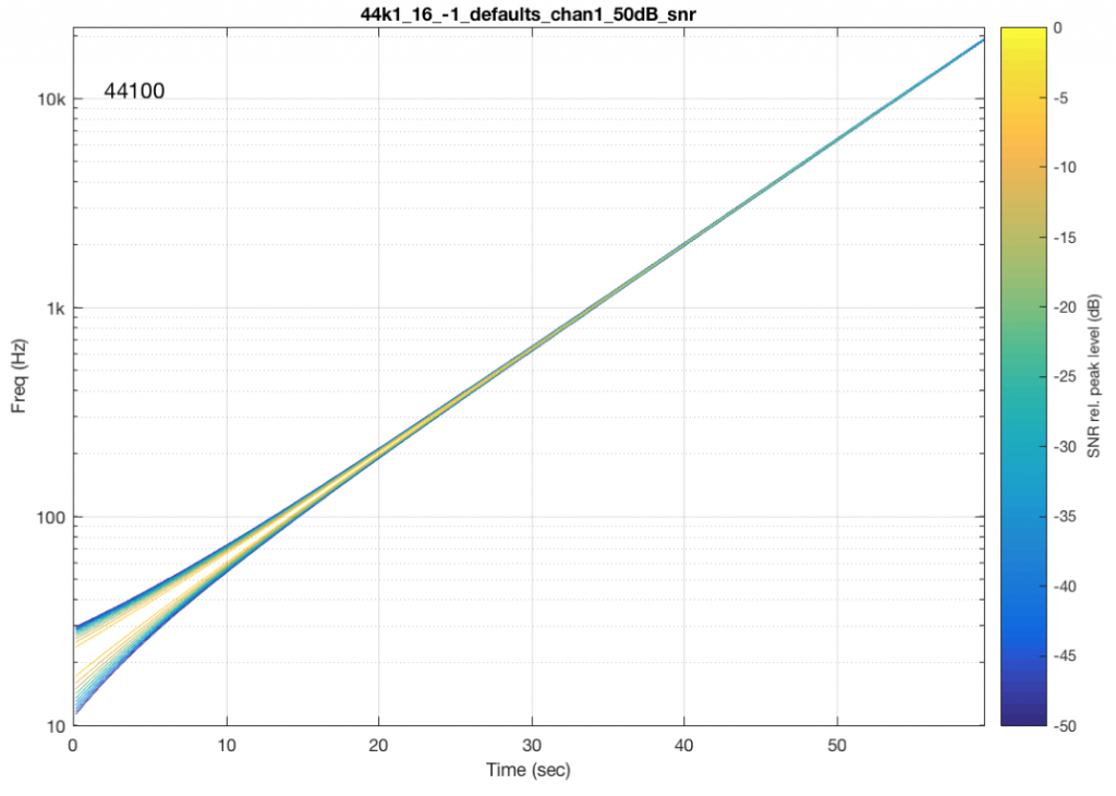
You may notice that the plot looks a little “wide” in the beginning. This is because the window length of the FFT I’m using to analyse the signal isn’t long enough to get a precise analysis of a low-frequency signal. So, this is an artefact of the analysis – not an error in the playback system.
What happens if we have random skip/insert events in the system? This is shown in Figure 7.
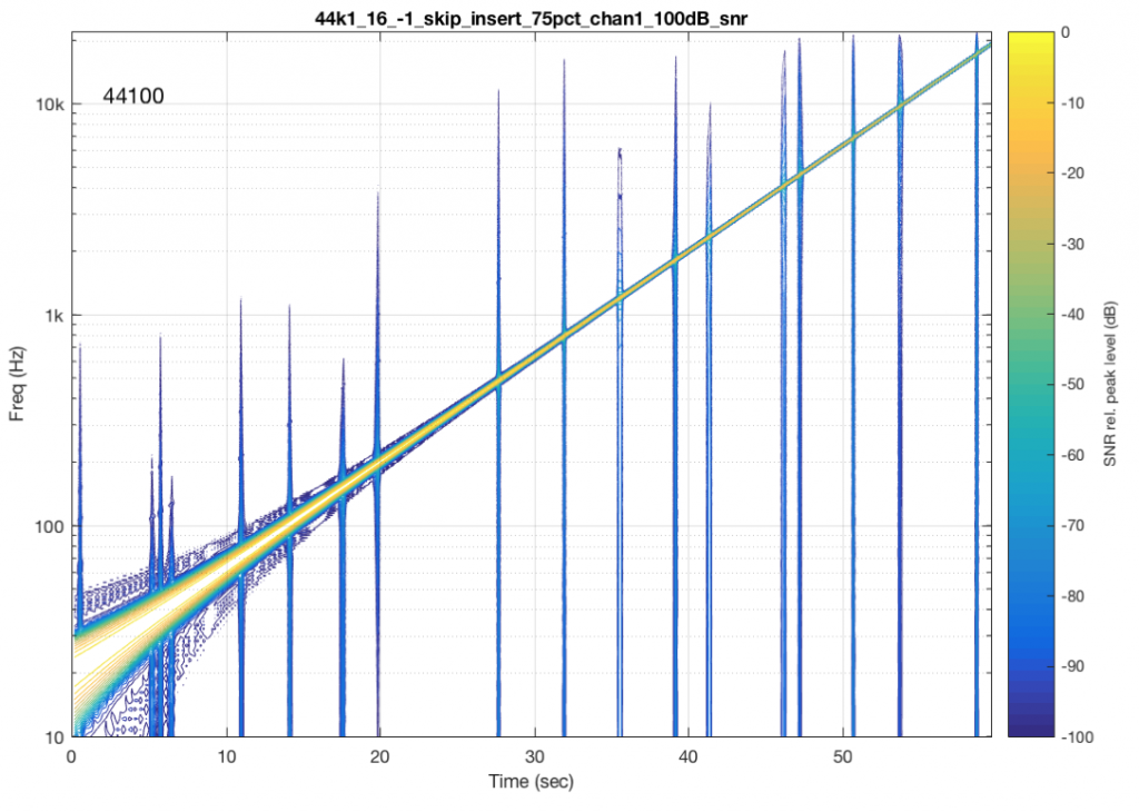
The signal in Figure 7 was one that I created – I intentionally made skip/insert events at random times and applied them to my test signal.
There are two things to notice here. The first is that each event is visible as a vertical “spike” in the plot. This is because a skip/insert event will cause a short, wide-band “burst” that sounds like a click. However, the bandwidth of the click is dependent on when it happens relative to the signal. For example, the skip/insert events in Figure 2 and 4 would not create as much high-frequency energy as the ones in Figure 3 and 5. So, the bigger the effect on the slope of the signal, the more high frequency energy we’ll get in our “click” sound. Since the slope of a signal increases with frequency, then this also means that low-frequency signals will likely produce lower-bandwidth artefacts.
Now let’s look at the results from some real-world devices and systems that are commercially available.
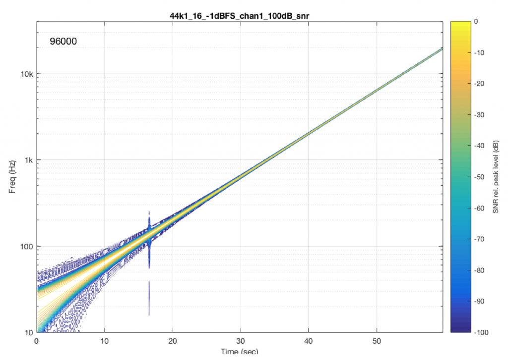
As you can see in Figure 8, there was one skip/insert event that happened during the 60 seconds I was running this test. Remember that the time that that event happened had nothing to do with the frequency it was playing. It just happens when it happens due to the relationship between the transmitter’s and the receiver’s clock speeds.
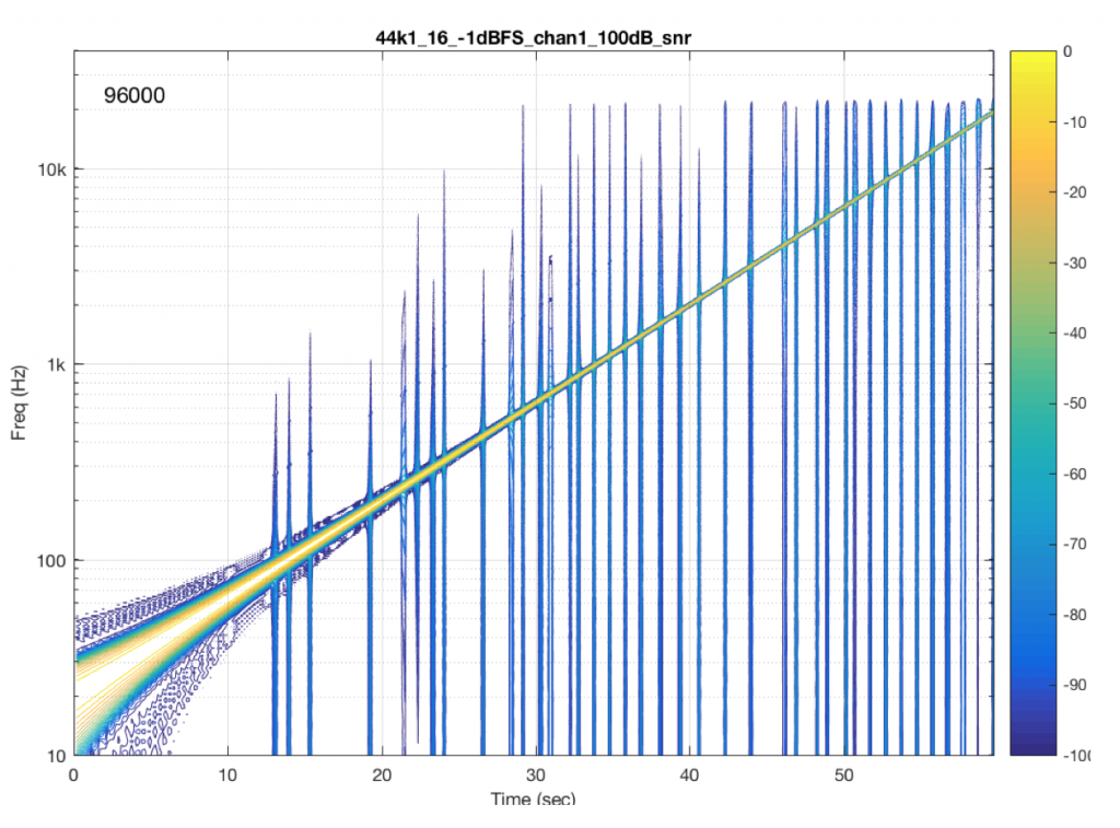
Figure 9 shows the results from a different system/device that obviously uses a skip/insert strategy to deal with clock synchronisation problems. It also obviously has some serious clock issues, since it has to correct on the order of approximately once a second…
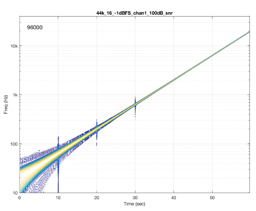
Figure 10 shows the results from a different system/device that uses a skip/insert strategy – but appears to do so at scheduled intervals. In this case, there is a high probability of getting a skip/insert event every 10 seconds with the counter starting at the instant I starting hearing the music.
Addendum 1
Inquisitive readers may be asking why it is that, although I’m doing an analysis down to -101 dB FS (100 dB below the signal level of -1 dB FS), you can’t see the effects of the dither noise floor in my original 16-bit file (which is normally assumed to be at -93 dB FS). This is because the -93 dB FS estimate of a dither signal assumes that you are looking at the total energy from the entire frequency band. The spectrograms above are based on FFT’s that split up the total frequency band into “slices” (called frequency bins) – and the total energy in each of these bins is less than the total energy in all of them (one person clapping is not as loud as 1000 people clapping at the same time…). If we wanted to see the dither noise, I would have had to set my analysis to go down approximately 30 dB lower – but the actual value for this is dependent on the relationship between the sampling rate, the window length of the FFT’s, and the windowing function that I’m using.
Addendum 2
Do not bother contacting me to ask which “commercially-available system/device” I measured and in which I found these errors. I’m not doing this to get anyone in trouble. I’m just doing this to try to illustrate common errors that I see often when I evaluate and test audio devices.
An besides, it would not be fair for me to rat on specific companies, systems, or devices, since, in some cases, these errors may have already been fixed with a firmware update, meaning that “naming names” would be irrelevant and unnecessarily detrimental.
But, I will say that I see this problem often. A rough estimate is that I would see errors like this on roughly half of the commercially-available devices and systems I test. It can also be sneaky, as we saw in Figures 8 and 10. Sometimes you get one of these clicks only once in a minute. So, if you do a 10-second measurement to test if your wireless audio receiver is “bit accurate” – the answer can be “yes” – but if you keep measuring for 1 or 2 minutes, you find out the answer is “no”…
Addendum 3
If it helps, I could have used the example of a leap year instead of two clocks at the beginning. The reason we have a February 29 every 4 years is that our calendar “runs” a little faster than the time it takes us to get around the sun (because a “year” is actually 365.25 days long…). So, every 4 years we have to “insert” a day to put the two clocks back in sync.
Also, since a “year” is not exactly 365.25 days long, we also have the occasional “leap second” as well. But most people don’t notice this, since it’s rarely useful as an excuse when you’ve missed a meeting…
Typical Errors in Digital Audio: Part 3 – Aliasing
Reminder: This is still just the lead-up to the real topic of this series. However, we have to get some basics out of the way first…
In the first posting in this series, I talked about digital audio (more accurately, Linear Pulse Code Modulation or LPCM digital audio) is basically just a string of stored measurements of the electrical voltage that is analogous to the audio signal, which is a change in pressure over time… In the second posting in the series, we looked at a “trick” for dealing with the issue of quantisation (the fact that we have a limited resolution for measuring the amplitude of the audio signal). This trick is to add dither (a fancy word for “noise”) to the signal before we quantise it in order to randomise the error and turn it into noise instead of distortion.
In this posting, we’ll look at some of the problems incurred by the way we carve up time into discrete moments when we grab those samples.
Let’s make a wheel that has one spoke. We’ll rotate it at some speed, and make a film of it turning. We can define the rotational speed in RPM – rotations per minute, but this is not very useful. In this case, what’s more useful is to measure the wheel rotation speed in degrees per frame of the film.
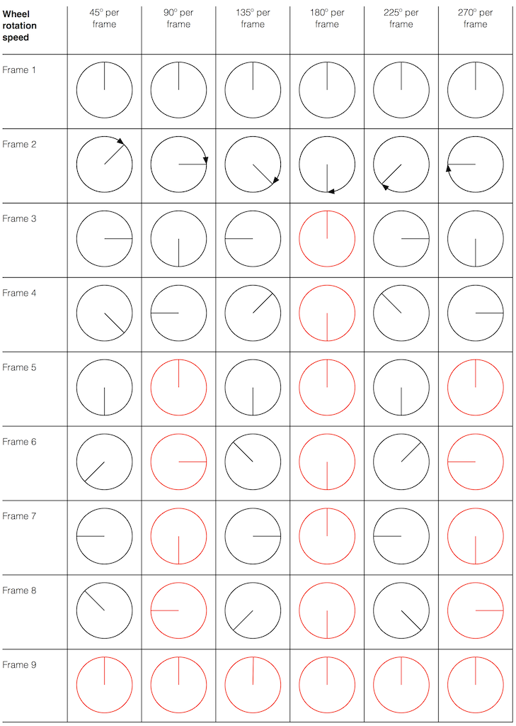
Take a look at the left-most column in Figure 1. This shows the wheel rotating 45º each frame. If we play back these frames, the wheel will look like it’s rotating 45º per frame. So, the playback of the wheel rotating looks the same as it does in real life.
This is more or less the same for the next two columns, showing rotational speeds of 90º and 135º per frame.
However, things change dramatically when we look at the next column – the wheel rotating at 180º per frame. Think about what this would look like if we played this movie (assuming that the frame rate is pretty fast – fast enough that we don’t see things blinking…) Instead of seeing a rotating wheel with only one spoke, we would see a wheel that’s not rotating – and with two spokes.
This is important, so let’s think about this some more. This means that, because we are cutting time into discrete moments (each frame is a “slice” of time) and at a regular rate (I’m assuming here that the frame rate of the film does not vary), then the movement of the wheel is recorded (since our 1 spoke turns into 2) but the direction of movement does not. (We don’t know whether the wheel is rotating clockwise or counter-clockwise. Both directions of rotation would result in the same film…)
Now, let’s move over one more column – where the wheel is rotating at 225º per frame. In this case, if we look at the film, it appears that the wheel is back to having only one spoke again – but it will appear to be rotating backwards at a rate of 135º per frame. So, although the wheel is rotating clockwise, the film shows it rotating counter-clockwise at a different (slower) speed. This is an effect that you’ve probably seen many times in films and on TV. What may come as a surprise is that this never happens in “real life” unless you’re in a place where the lights are flickering at a constant rate (as in the case of fluorescent or some LED lights, for example).
Again, we have to consider the fact that if the wheel actually were rotating counter-clockwise at 135º per frame, we would get exactly the same thing on the frames of the film as when the wheel if rotating clockwise at 225º per frame. These two events in real life will result in identical photos in the film. This is important – so if it didn’t make sense, read it again.
This means that, if all you know is what’s on the film, you cannot determine whether the wheel was going clockwise at 225º per frame, or counter-clockwise at 135º per frame. Both of these conclusions are valid interpretations of the “data” (the film). (Of course, there are more – the wheel could have rotated clockwise by 360º+225º = 585º or counter-clockwise by 360º+135º = 495º, for example…)
Since these two interpretations of reality are equally valid, we call the one we know is wrong an alias of the correct answer. If I say “The Big Apple”, most people will know that this is the same as saying “New York City” – it’s an alias that can be interpreted to mean the same thing.
Wheels and Slinkies
We people in audio commit many sins. One of them is that, every time we draw a plot of anything called “audio” we start out by drawing a sine wave. (A similar sin is committed by musicians who, at the first opportunity to play a grand piano, will play a middle-C, as if there were other notes in the world.) The question is: what, exactly, is a sine wave?
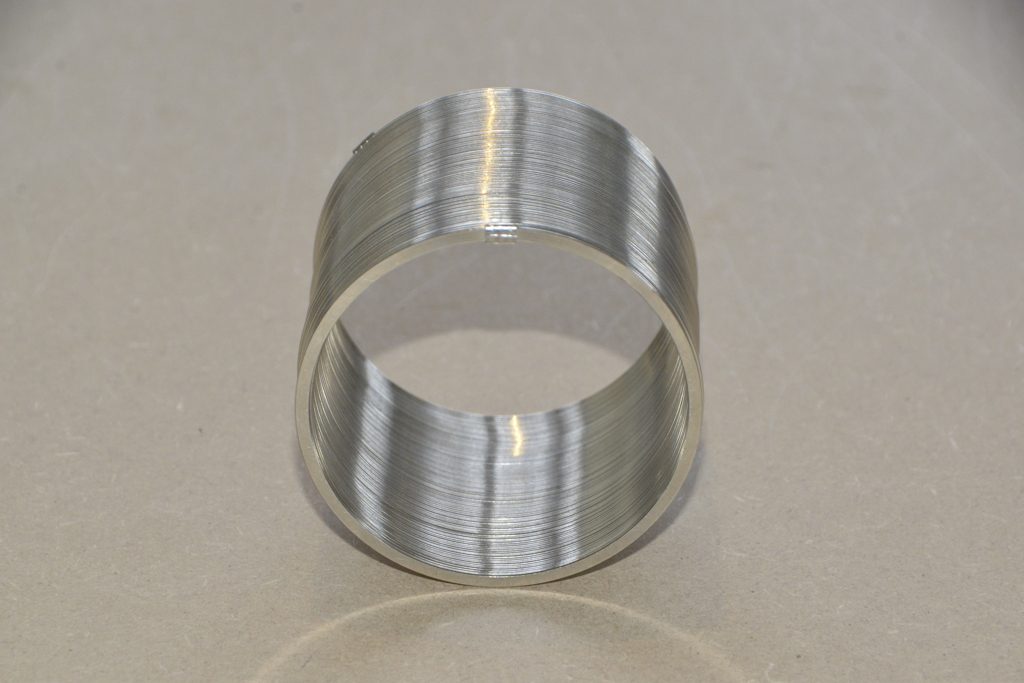
Get a Slinky – or if you don’t want to spend money on a brand name, get a spring. Look at it from one end, and you’ll see that it’s a circle, as can be (sort of) seen in Figure 2.
Since this is a circle, we can put marks on the Slinky at various amounts of rotation, as in Figure 3.
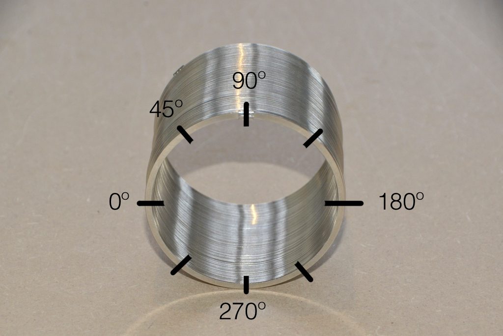
Of course, I could have put the 0º marl anywhere. I could have also rotated counter-clockwise instead of clockwise. But since both of these are arbitrary choices, I’m not going to debate either one.
Now, let’s rotate the Slinky so that we’re looking at from the side. We’ll stretch it out a little too…
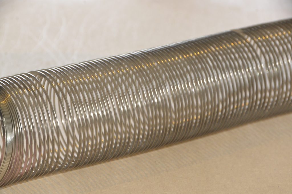
Let’s do that some more…
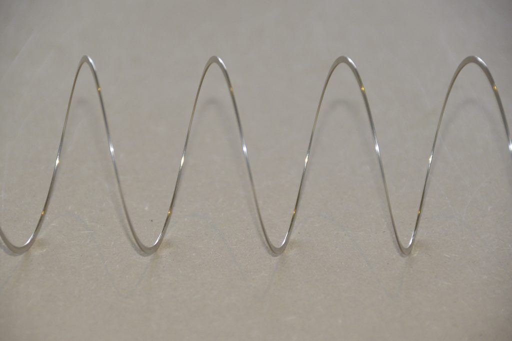
When you do this, and you look at the Slinky directly from one side, you are able to see the vertical change of the spring from the centre as a result of the change in rotation. For example, we can see in Figure 6 that, if you mark the 45º rotation point in this view, the distance from the centre of the spring is 71% of the maximum height of the spring (at 90º).
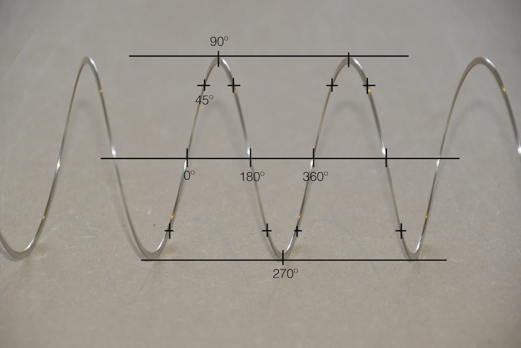
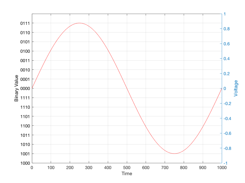
So what? Well, basically, the “punch line” here is that a sine wave is actually a “side view” of a rotation. So, Figure 7, shows a measurement – a capture – of the amplitude of the signal every 45º.
Since we can now think of a sine wave as a rotation of a circle viewed from the side, it should be just a small leap to see that Figure 7 and the left-most column of Figure 1 are basically identical.
Let’s make audio equivalents of the different columns in Figure 1.
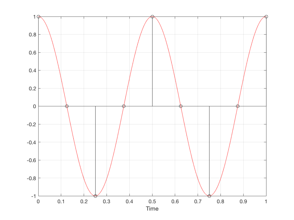
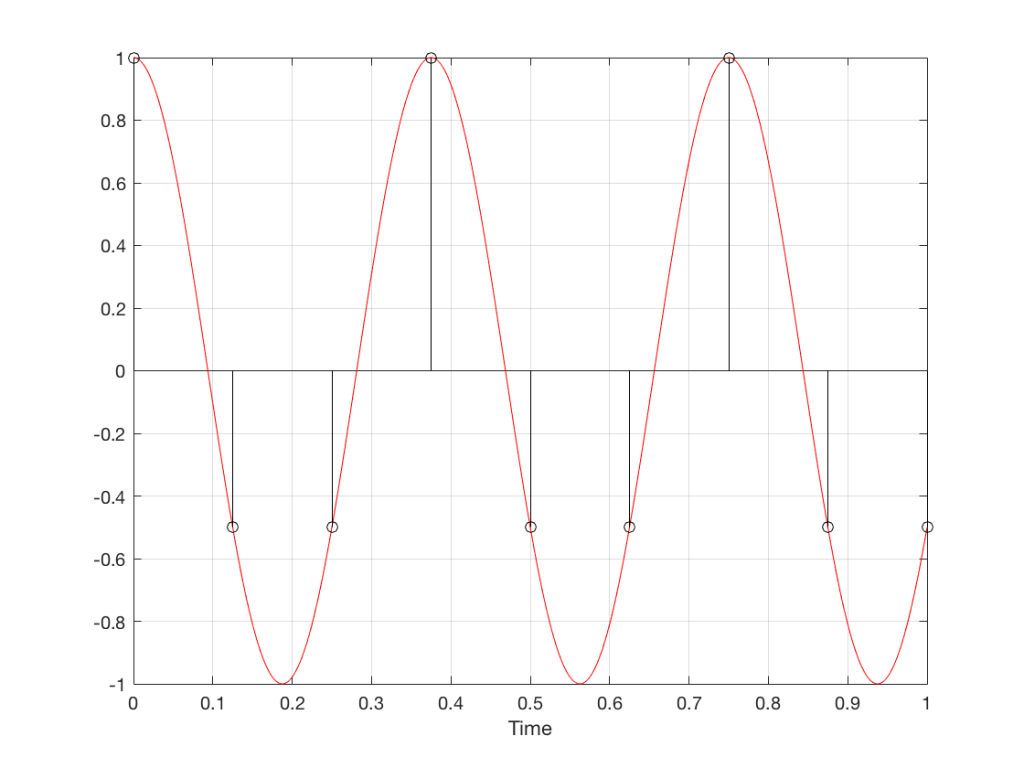
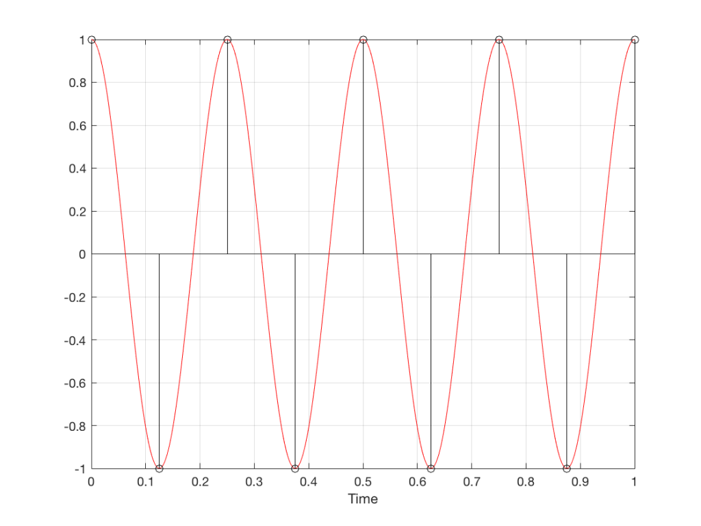
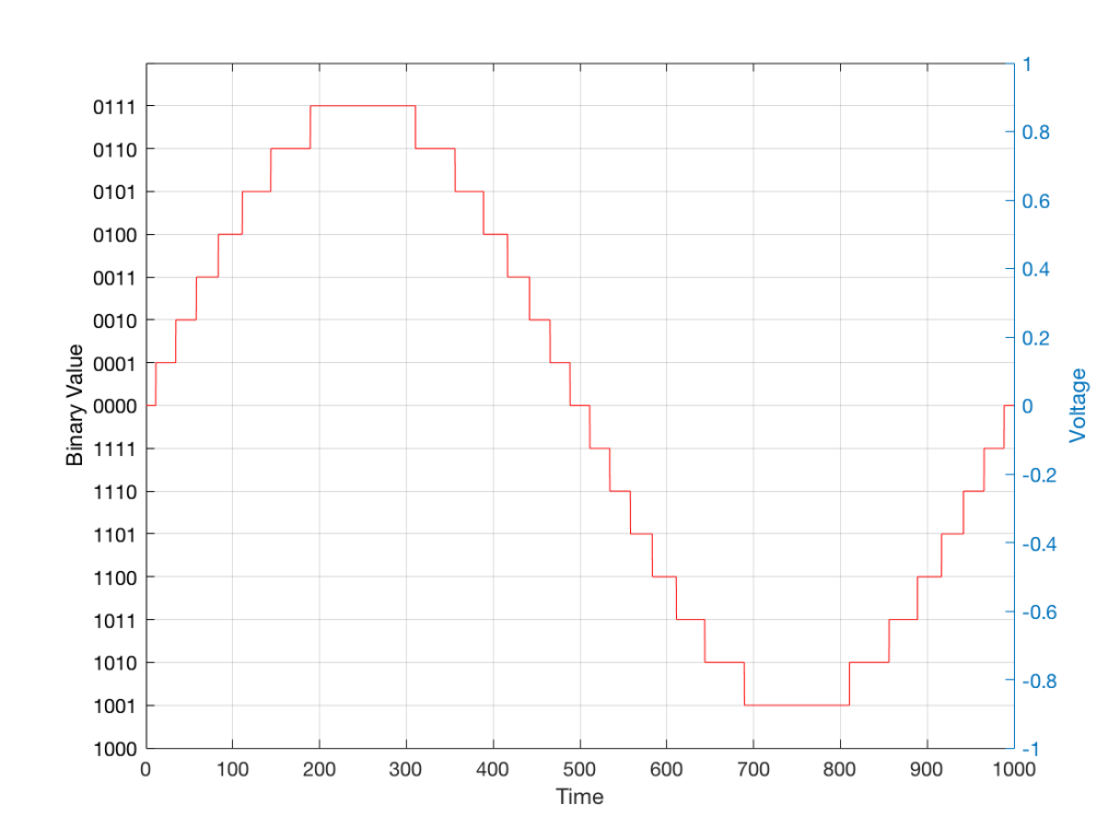
Figure 10 is an important one. Notice that we have a case here where there are exactly 2 samples per period of the cosine wave. This means that our sampling frequency (the number of samples we make per second) is exactly one-half of the frequency of the signal. If the signal gets any higher in frequency than this, then we will be making fewer than 2 samples per period. And, as we saw in Figure 1, this is where things start to go haywire.
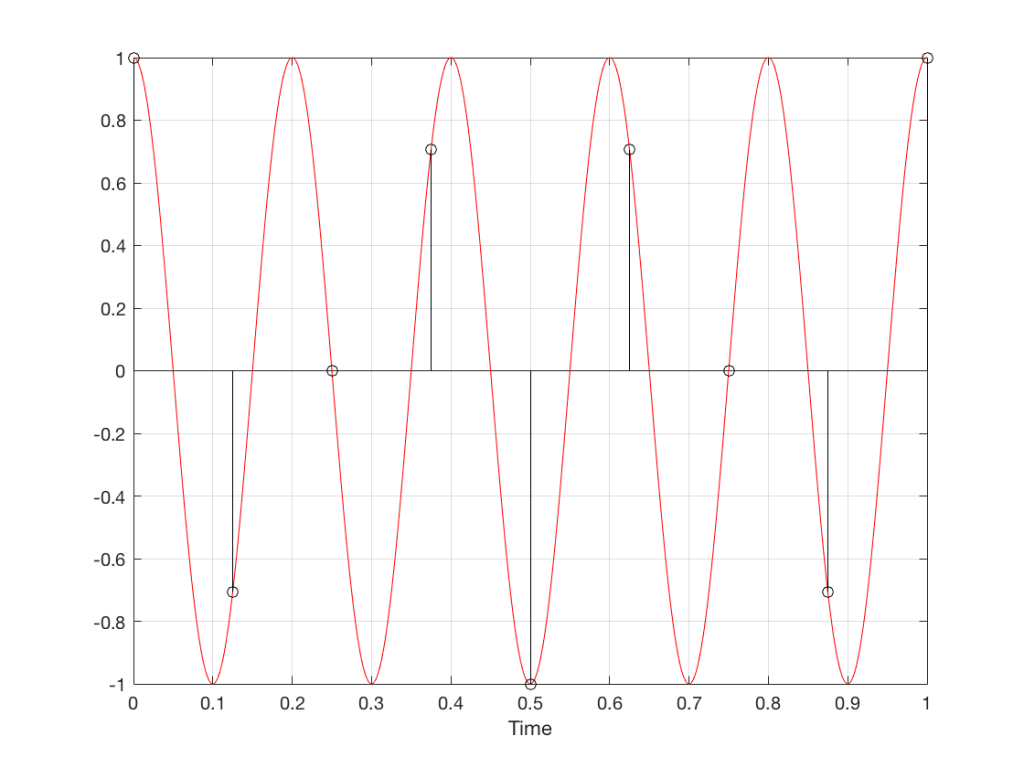
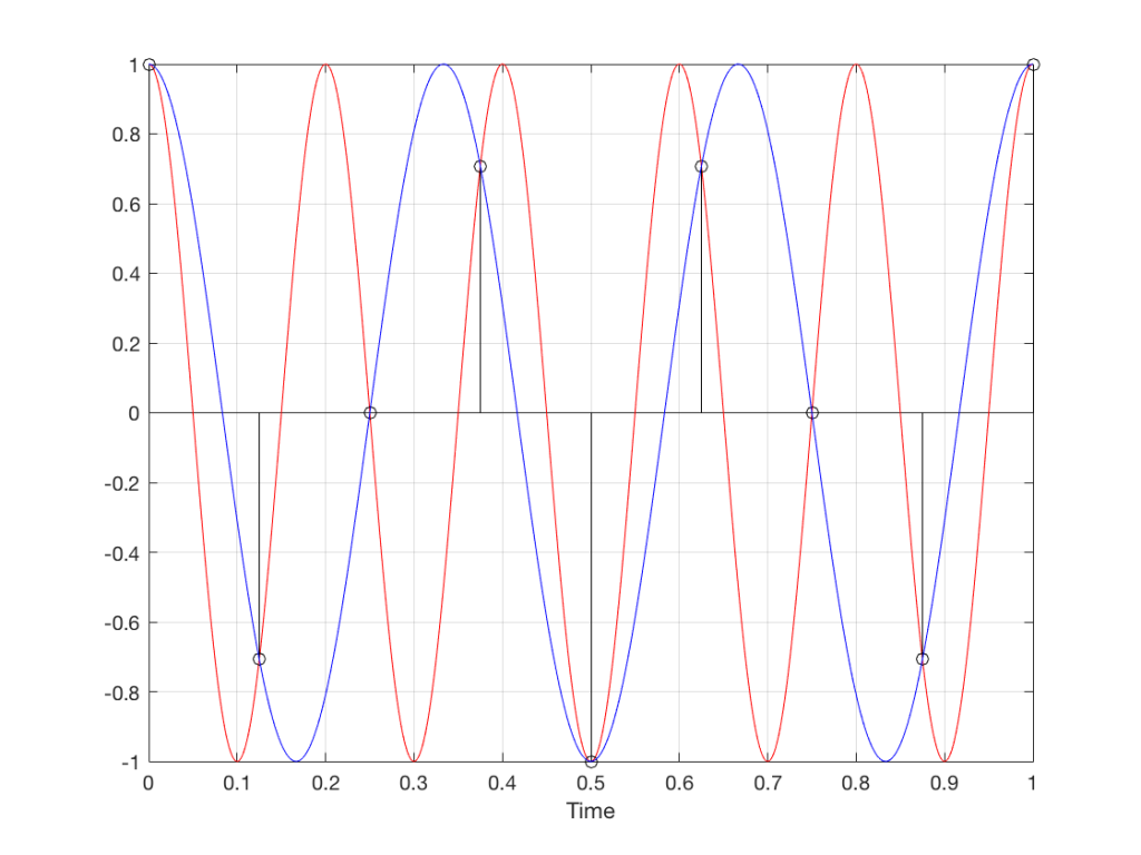
Figure 11 shows the equivalent audio case to the “225º per frame” column in Figure 1. When we were talking about rotating wheels, we saw that this resulted in a film that looked like the wheel was rotating backwards at the wrong speed. The audio equivalent of this “wrong speed” is “a different frequency” – the alias of the actual frequency. However, we have to remember that both the correct frequency and the alias are valid answers – so, in fact, both frequencies (or, more accurately, all of the frequencies) exist in the signal.
So, we could take Fig 11, look at the samples (the black lollipops) and figure out what other frequency fits these. That’s shown in Figure 12.
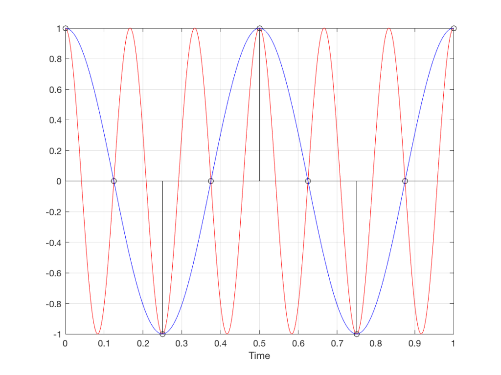
Moving up in frequency one more step, we get to the right-hand column in Figure 1, whose equivalent, including the aliased signal, are shown in Figure 13.
Do I need to worry yet?
Hopefully, now, you can see that an LPCM system has a limit with respect to the maximum frequency that it can deal with appropriately. Specifically, the signal that you are trying to capture CANNOT exceed one-half of the sampling rate. So, if you are recording a CD, which has a sampling rate of 44,100 samples per second (or 44.1 kHz) then you CANNOT have any audio signals in that system that are higher than 22,050 Hz.
That limit is commonly known as the “Nyquist frequency“, named after Harry Nyquist – one of the persons who figured out that this limit exists.
In theory, this is always true. So, when someone did the recording destined for the CD, they made sure that the signal went through a low-pass filter that eliminated all signals above the Nyquist frequency.
In practice, however, there are many cases where aliasing occurs in digital audio systems because someone wasn’t paying enough attention to what was happening “under the hood” in the signal processing of an audio device. This will come up later.
Two more details to remember…
There’s an easy way to predict the output of a system that’s suffering from aliasing if your input is sinusoidal (and therefore contains only one frequency). The frequency of the output signal will be the same distance from the Nyquist frequency as the frequency if the input signal. In other words, the Nyquist frequency is like a “mirror” that “reflects” the frequency of the input signal to another frequency below Nyquist.
This can be easily seen in the upper plot of Figure 14. The distance from the Input signal and the Nyquist is the same as the distance between the output signal and the Nyquist.
Also, since that Nyquist frequency acts as a mirror, then the Input and output signal’s frequencies will move in opposite directions (this point will help later).
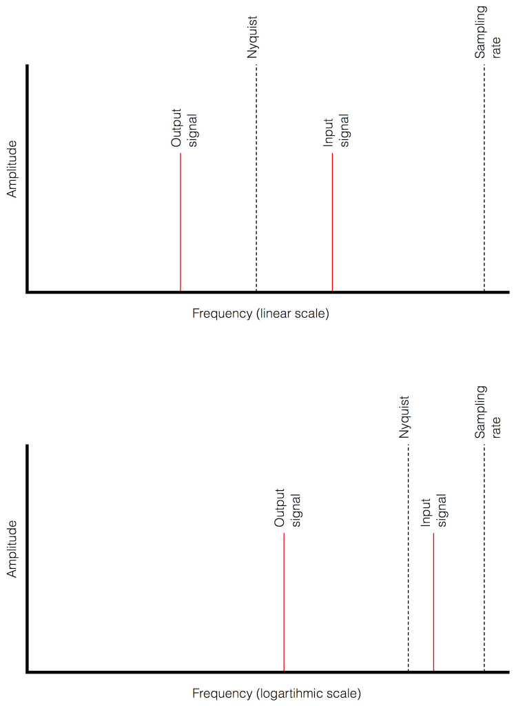
Usually, frequency-domain plots are done on a logarithmic scale, because this is more intuitive for we humans who hear logarithmically. (For example, we hear two consecutive octaves on a piano as having the same “interval” or “width”. We don’t hear the width of the upper octave as being twice as wide, like a measurement system does. that’s why music notation does not get wider on the top, with a really tall treble clef.) This means that it’s not as obvious that the Nyquist frequency is in the centre of the frequencies of the input signal and its alias below Nyquist.
Typical Errors in Digital Audio: Part 2 – Dither
Reminder: This is still just the lead-up to the real topic of this series. However, we have to get some basics out of the way first…
In the last posting, I talked about digital audio (more accurately, Linear Pulse Code Modulation or LPCM digital audio) is basically just a string of stored measurements of the electrical voltage that is analogous to the audio signal, which is a change in pressure over time…
For now, we’ll say that each measurement is rounded off to the nearest possible “tick” on the ruler that we’re using to measure the voltage. That rounding results in an error. However, (assuming that everything is working correctly) that error can never be bigger than 1/2 of a “step”. Therefore, in order to reduce the amount of error, we need to increase the number of ticks on the ruler.
Now we have to introduce a new word. If we really had a ruler, we could talk about whether the ticks are 1 mm apart – or 1/16″ – or whatever. We talk about the resolution of the ruler in terms of distance between ticks. However, if we are going to be more general, we can talk about the distance between two ticks being one “quantum” – a fancy word for the smallest step size on the ruler.
So, when you’re “rounding off to the nearest value” you are “quantising” the measurement (or “quantizing” it, if you live in Noah Webster’s country and therefore you harbor the belief that wordz should be spelled like they sound – and therefore the world needz more zees). This also means that the amount of error that you get as a result of that “rounding off” is called “quantisation error“.
In some explanations of this problem, you may read that this error is called “quantisation noise”. However, this isn’t always correct. This is because if something is “noise” then is is random, and therefore impossible to predict. However, that’s not strictly the case for quantisation error. If you know the signal, and you know the quantisation values, then you’ll be able to predict exactly what the error will be. So, although that error might sound like noise, technically speaking, it’s not. This can easily be seen in Figures 1 through 3 which demonstrate that the quantisation error causes a periodic, predictable error (and therefore harmonic distortion), not a random error (and therefore noise).
Sidebar: The reason people call it quantisation noise is that, if the signal is complicated (unlike a sine wave) and high in level relative to the quantisation levels – say a recording of Britney Spears, for example – then the distortion that is generated sounds “random-ish”, which causes people to just to the conclusion that it’s noise.
Now, let’s talk about perception for a while… We humans are really good at detecting patterns – signals – in an otherwise noisy world. This is just as true with hearing as it is with vision. So, if you have a sound that exists in a truly random background noise, then you can focus on listening to the sound and ignore the noise. For example, if you (like me) are old enough to have used cassette tapes, then you can remember listening to songs with a high background noise (the “tape hiss”) – but it wasn’t too annoying because the hiss was independent of the music, and constant. However, if you, like me, have listened to Bob Marley’s live version of “No Woman No Cry” from the “Legend” album, then you, like me, would miss the the feedback in the PA system at that point in the song when the FoH engineer wasn’t paying enough attention… That noise (the howl of the feedback) is not noise – it’s a signal… Which makes it just as important as the song itself. (I could get into a long boring talk about John Cage at this point, but I’ll try to not get too distracted…)
The problem with the signal in Figure 2 is that the error (shown in Figure 3) is periodic – it’s a signal that demands attention. If the signal that I was sending into the quantisation system (in Figure 1) was a little more complicated than a sine wave – say a sine wave with an amplitude modulation – then the error would be easily “trackable” by anyone who was listening.
So, what we want to do is to quantise the signal (because we’re assuming that we can’t make a better “ruler”) but to make the error random – so it is changed from distortion to noise. We do this by adding noise to the signal before we quantise it. The result of this is that the error will be randomised, and will become independent of the original signal… So, instead of a modulating signal with modulated distortion, we get a modulated signal with constant noise – which is easier for us to ignore. (It has the added benefit of spreading the frequency content of the error over a wide frequency band, rather than being stuck on the harmonics of the original signal… but let’s not talk about that…)
For example…
Let’s take a look at an example of this from an equivalent world – digital photography.
The photo in Figure 4 is a black and white photo – which actually means that it’s comprised of shades of gray ranging from black all the way to white. The photo has 272,640 individual pixels (because it’s 640 pixels wide and 426 pixels high). Each of those pixels is some shade of gray, but that shading does not have an infinite resolution. There are “only” 256 possible shades of gray available for each pixel.
So, each pixel has a number that can range from 0 (black) up to 255 (white).

If we were to zoom in to the top left corner of the photo and look at the values of the 64 pixels there (an 8×8 pixel square), you’d see that they are:
86 86 90 88 87 87 90 91
86 88 90 90 89 87 90 91
88 89 91 90 89 89 90 94
88 90 91 93 90 90 93 94
89 93 94 94 91 93 94 96
90 93 94 95 94 91 95 96
93 94 97 95 94 95 96 97
93 94 97 97 96 94 97 97
What if we were to reduce the available resolution so that there were fewer shades of gray between white and black? We can take the photo in Figure 1 and round the value in each pixel to the new value. For example, Figure 5 shows an example of the same photo reduced to only 4 levels of gray.

Now, if we look at those same pixels in the upper left corner, we’d see that their values are
102 102 102 102 102 102 102 102
102 102 102 102 102 102 102 102
102 102 102 102 102 102 102 102
102 102 102 102 102 102 102 102
102 102 102 102 102 102 102 102
102 102 102 102 102 102 102 102
102 102 102 102 102 102 102 102
102 102 102 102 102 102 102 102
They’ve all been quantised to the nearest available level, which is 102. (Our possible values are restricted to 0, 51, 102, 154, 205, and 255).
So, we can see that, by quantising the gray levels from 256 possible values down to only 6, we lose details in the photo. This should not be a surprise… That loss of detail means that, for example, the gentle transition from lighter to darker gray in the sky in the original is “flattened” to a light spot in a darker background, with a jagged edge at the transition between the two. Also, the details of the wall pillars between the windows are lost.
If we take our original photo and add noise to it – so were adding a random value to the value of each pixel in the original photo (I won’t talk about the range of those random values…) it will look like Figure 6. This photo has all 256 possible values of gray – the same as in Figure 1.

If we then quantise Figure 6 using our 6 possible values of gray, we get Figure 7. Notice that, although we do not have more grays than in Figure 5, we can see things like the gradual shading in the sky and some details in the walls between the tall windows.

That noise that we add to the original signal is called dither – because it is forcing the quantiser to be indecisive about which level to quantise to choose.
I should be clear here and say that dither does not eliminate quantisation error. The purpose of dither is to randomise the error, turning the quantisation error into noise instead of distortion. This makes it (among other things) independent of the signal that you’re listening to, so it’s easier for your brain to separate it from the music, and ignore it.
Addendum: Binary basics and SNR
We normally write down our numbers using a “base 10” notation. So, when I write down 9374 – I mean
9 x 1000 + 3 x 100 + 7 x 10 + 4 x 1
or
9 x 10³ + 3 x 10² + 7 x 101 + 4 x 100
We use base 10 notation – a system based on 10 digits (0 through 9) because we have 10 fingers.
If we only had 2 fingers, we would do things differently… We would only have 2 digits (0 and 1) and we would write down numbers like this:
11101
which would be the same as saying
1 x 16 + 1 x 8 + 1 x 4 + 0 x 2 + 1 x 1
or
1 x 24 + 1 x 23 + 1 x 22 + 0 x 21 + 1 x 20
The details of this are not important – but one small point is. If we’re using a base-10 system and we increase the number by one more digit – say, going from a 3-digit number to a 4-digit number, then we increase the possible number of values we can represent by a factor of 10. (in other words, there are 10 times as many possible values in the number XXXX than in XXX.)
If we’re using a base-2 system and we increase by one extra digit, we increase the number of possible values by a factor of 2. So XXXX has 2 times as many possible values as XXX.
Now, remember that the error that we generate when we quantise is no bigger than 1/2 of a quantisation step, regardless of the number of steps. So, if we double the number of steps (by adding an extra binary digit or bit to the value that we’re storing), then the signal can be twice as “far away” from the quantisation error.
This means that, by adding an extra bit to the stored value, we increase the potential signal-to-error ratio of our LPCM system by a factor of 2 – or 6.02 dB.
So, if we have a 16-bit LPCM signal, then a sine wave at the maximum level that it can be without clipping is about 6 dB/bit * 16 bits – 3 dB = 93 dB louder than the error. The reason we subtract the 3 dB from the value is that the error is +/- 0.5 of a quantisation step (normally called an “LSB” or “Least Significant Bit”).
Note as well that this calculation is just a rule of thumb. It is neither precise nor accurate, since the details of exactly what kind of error we have will have a minor effect on the actual number. However, it will be close enough.