Before starting on this portion of the series, I’ll ask you to think about how little energy (or movement) it takes to get a resonant system oscillating. For example, if you have a child on a swing, a series of very gentle pushes at the right times can result in them swinging very high. Also, once the child is swinging back and forth, it takes a lot of effort to stop them quickly.
Moving onwards…
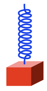
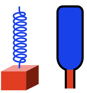
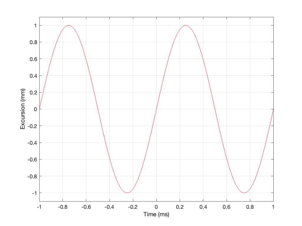
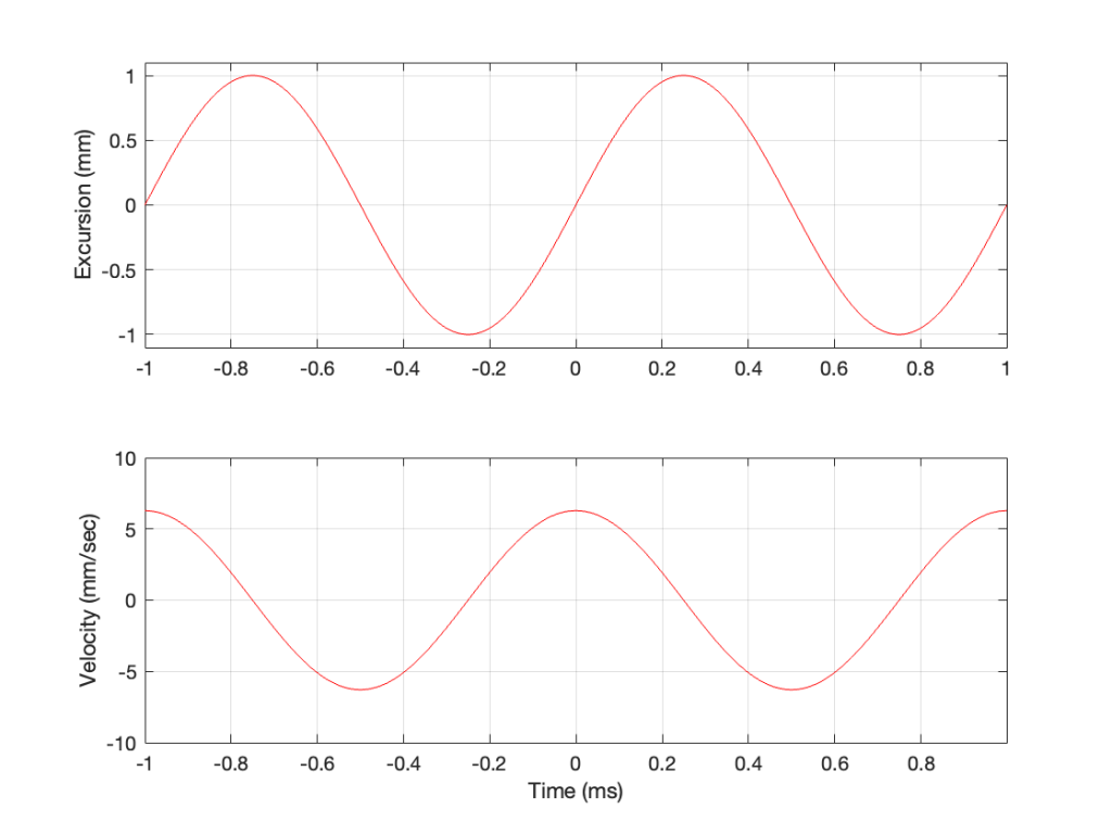
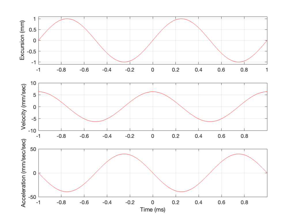
So far, we’ve seen that a loudspeaker driver in a closed cabinet can be thought of as just a mass on a spring, and, as a result, it has some natural resonance where it will oscillate at some frequency.
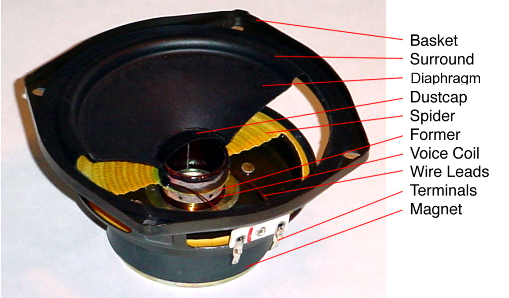
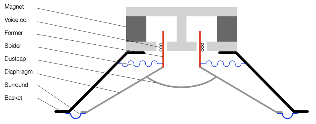
The driver is normally moved by sending an electrical signal into its voice coil. This causes the coil to produce a magnetic field and, since it’s already sitting in the magnetic field of a permanent magnet, it moves. The surround and spider prevent it from moving sideways, so it can only move outwards (if we send electrical current in one direction) or inwards (if we send current in the other direction).
When you try to move the driver, you’re working against a number of things:
- the inertia of the mass of the moving parts
Pick up a heavy book, for example, and try to push and pull it back and forth. It’s hard work! - the inertia of the air directly in front of and behind the driver
Pick up a big sheet of stiff plastic (like the thing you put on the floor under an office chair) and try to push it back and forth. It’s also hard work! - the compliance (springiness) of the surround, spider, and air trapped in the cabinet behind the driver
Blow up a ballon, and use your two hands to squeeze it repeatedly. It’s also hard work!
These three things can be considered separately from each other as a static effect. In other words:
- It’s hard work to pick up a book or push a car that’s broken down (forget about pushing-and-pulling – just push OR pull)
- It’s hard work to run into a headwind with that big piece of stiff plastic
- It’s hard work to squeeze a balloon and keep it compressed
But, if you’re pushing AND pulling the loudspeaker driver there is another effect that’s dynamic.
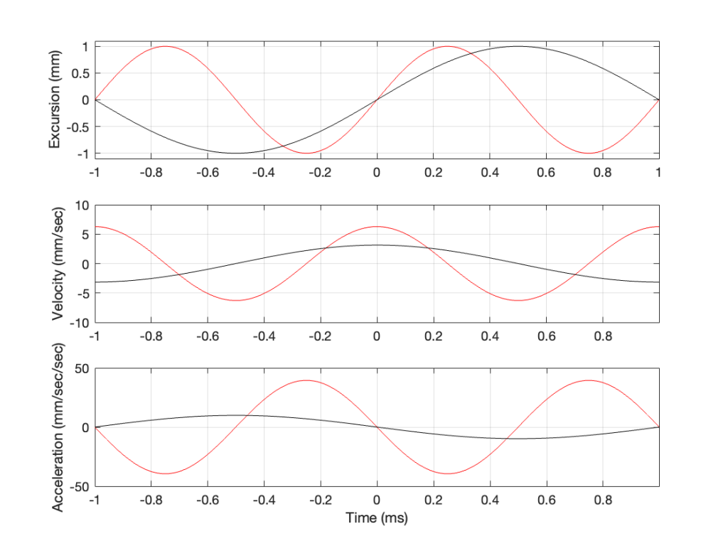
When you’re moving the driver at a VERY low frequency, you’re mostly working against the “spring” which is probably quite easy to do. So, at a low frequency, the driver is pretty easy to move, and it’s moving so slowly that it doesn’t push back electrically. So, it does not impede the flow of current through the voice coil.
When you’re moving the driver at a VERY high frequency, you’re mostly working against the inertia of the moving parts and the adjacent air molecules. The higher the frequency, the harder it is to move the driver.
However, when you’re trying to moving the driver at exactly the resonant frequency of the driver, you don’t need much energy at all because it “wants” to move at that same rate. However, at that frequency, the voice coil is moving in the magnetic field of the permanent magnet, and it generates electricity that is trying to move current in the opposite direction of what your amp is going. In other words, at the driver’s resonant frequency, when you’re trying to push current into the voice coil, it generates a current that pushes back. When you try to pull current out of the voice coil, it generates a current that pulls back.
In other words, at the driver’s resonant frequency, your amplifier “sees” the driver as as a thing that is trying to impede the flow of electrical current. This means that you get a lot of movement with only a little electrical current; just like the child on the swing gets to go high with only a little effort – but only at one frequency.
This is a nice, simple case where you have a moving mass (the moving parts of the driver) and a spring (the surround, spider, and air in the sealed box). But what happens when the speaker has a port?
On to Part 4…