
What’s even more interesting is to know that they named it “Deep note” after “Deep thought” from HHGG… Small things make me happy.
What’s even more interesting is to know that they named it “Deep note” after “Deep thought” from HHGG… Small things make me happy.
#37 in a series of articles about the technology behind Bang & Olufsen loudspeakers
In the last posting, I described a little experiment that we did where we could easily be accused of asking a stupid question and getting an obvious answer. This posting is a little different, although I’ll also describe a little experiment where we asked a much-less-stupid question and got an answer we weren’t looking for… However, before I describe the experiment itself, we’ll have to start with a little background information.
Let’s say that we wanted to build a “simple” two-way loudspeaker with a tweeter and a woofer in a box like the one shown in Figure 1.

Since we’re Bang & Olufsen, it is implied that this will be a fully active, DSP-based loudspeaker. Let’s also, for the sake of simplicity, say that we used loudspeaker drivers and other components with absolutely no linear distortion artefacts (I can dream, can’t I?). This means that we can apply any kind of filter we like to each of the two loudspeaker drivers to result in whatever response we want (in a given direction in a “free field” (a space with no reflecting surfaces, extending to infinity in all directions) – for more information on this, please read this posting and/or this posting).
Now, it’s fairly reasonable to assume that one portion of a good starting point for a loudspeaker’s acoustic response is to have a flat magnitude response when measured on-axis in a free field. This means that, if you have the loudspeaker in a space that has no reflections, and you are directly in front of it, no frequency will be louder than any other (within some limits, of course…). In fact, this is the way a lot of studio monitor loudspeakers are tuned (which makes sense, since many studio control rooms don’t have a lot of reflections as was discussed here).
The problem is that, if you do make a loudspeaker that is flat-on-axis, you’ll probably have problems in its power response (for a description of what a loudspeaker’s “power response” is, see here). This is dependent on a lot of things like the crossover frequency, the sizes and shapes of the drivers, the phase responses of the crossover filters, the shape of the cabinet, and other things. However, if we were to simplify, we could say that a two-way loudspeaker (say, with a 4th order Linkwitz-Riley crossover, just to pick one type…) that is flat on-axis, will have a dip in its power response at the crossover frequency. This is because, although the two drivers (the tweeter and the woofer) add together nicely in one location (on-axis, directly in front of the loudspeaker) they do not add together nicely anywhere else (because the distances to the two drivers from the listening position are probably not matched, particularly when you go vertical…).
So, one basic problem with building a “simple” two-way loudspeaker is that you have to choose to either have a flat magnitude response on-axis, or a smooth power response (without a dip) – but you can’t have both. (If you want to really dig into this, I’d recommend starting with J. Vanderkooy & S.P. Lipshitz, “Power Response of Loudspeakers with Noncoincident Drivers — The Influence of Crossover Design,” J. Audio Eng. Soc., Vol. 34, No. 4, pp. 236-244 (Apr. 1986).)
This basic problem raised a question in the head of one of our acoustical engineers, Gert Munch. He started to wonder how we could build a loudspeaker that could have a flat magnitude response on-axis and still have a smooth power response that didn’t suffer from a dip at the crossover. One possible solution is to build a loudspeaker with the desired on-axis response, and then somehow create an additional portion of the loudspeaker that could “fill up” the dip in the power response by sending energy into the room without it affecting the on-axis response.
One possible way to do this is to use an extra loudspeaker with a “dipole” characteristic – a two-sided loudspeaker where the same signal is sent to both sides, but in opposite polarity. This means that, when one side of the loudspeaker produces a high pressure, the other side produces a low. When you sit on one side of the loudspeaker or the other, then you hear a signal. However, if you sit “on edge” to the loudspeaker, you hear nothing, since the two sides of the loudspeaker cancel each other out (in theory).
So, Gert’s idea was to add a two-way dipole loudspeaker on the top of a normal two-way loudspeaker and to just use the dipole (which became known as a “shark fin” – shown in Figure 2) to add energy around the crossover frequency of the “normal” loudspeaker. Since the edge of the dipole was facing forwards, the theory was that none of its sound would have an effect on the on-axis response of the two-way loudspeaker below it.

So, the question to answer was:
“Which sounds better:
?”
Since each of the 6 loudspeaker drivers in our model loudspeaker was independently controllable, this was an easy comparison to do on-the-fly, so we tried it out.
Also, just to be certain, we tried two different orientations of the dipole, both of which had the “null” – the edge of the loudspeaker – facing the listening position. The first orientation is shown in Figures 2 and 3. The second orientation is shown in Figure 4.


So, a bunch of us sat in the listening room for a week or so, listening to the various possible tunings of the loudspeakers, in various positions in the room, with various types of music. We each had an opinion about the whether we liked one configuration more or less than another. However, one thing that was noticeable was that there was an effect not only on the timbral impression of the loudspeakers (the tone colour) – but also on the spatial presentation of the pair. As we switched between the different tunings, phantom images changed in width and distance, and envelopment (when it existed in the recording) also changed.
This was particularly noticeable when the loudspeakers were closer to a reflecting surface, as is shown in Figure 5.

The end result was a bunch of different conclusions:
All of those little conclusions could be folded into two big ones:
So, this is where the concept of the shark fin died, but where the idea of “Beam Width Control” began.
Well… more accurately: it was the beginning of our thinking that being able to change the beam width (or the “directivity”, if you’re a geek) of the loudspeaker would be a useful “handle” in the hands of our customers. The idea that was born was something along the lines of the following: “If a customer could change the beam width of a loudspeaker, then (s)he could change it from being a narrow-directivity loudspeaker for people with one chair and no friends to a wide-directivity loudspeaker for people with a sofa and some friends to an omni-directivity loudspeaker for people throwing a party – all just by the flick of a switch…”
For more information on Beam Width Control:
#36 in a series of articles about the technology behind Bang & Olufsen loudspeakers
“In all affairs it’s a healthy thing now and then to hang a question mark on the things you have long taken for granted.”
-Bertrand Russell
If you were to get your hands on Harry Potter’s invisibility cloak and you were to walk into the acoustics department at Bang & Olufsen and eavesdrop on conversations, you’d sometimes be amazed at some of the questions we ask each other. That’s particularly true when we’re working on a new concept, because, if the concept is new, then it’s also new for us. The good thing is that all of my colleagues (and I) are ready and willing at any time to ask what might be considered to be a stupid (or at least a very basic) question.
One of those questions that we asked each other recently seemed like a basic one – why do we always put the tweeter on the top? It seems like there are very few loudspeakers that don’t do this (of course, there are exceptions – take the BeoLab Penta, for example, which has the tweeter in the middle). However, more often than not, when we (and most other people) make a loudspeaker, we put the loudspeaker drivers in ascending order of frequency – woofers on the bottom, tweeters on the top. Maybe this is because woofers are heavier, and if you stand a BeoLab 5 on its head, it will fall over – but that’s not really the question we were asking…
The REAL question we were asking ourselves at the time was: if we were to build a multi-way loudspeaker – let’s say a 3-way, with a woofer, a midrange and a tweeter, and if the crossovers were such that the bulk of the “interesting” information (say, the vocal range) was coming from the midrange, then why would we not put the midrange at ear height and put the tweeter between it and the woofer? For example, imagine we made BeoLab 20 without an Acoustic Lens on top, would it be better to arrange the drivers like the version on the left of Figure 1 or the version on the right? Which one would sound better?

After answering that question, there’s a second question would follow closely behind: how close together do the drivers with adjacent frequency bands (i.e. the woofer and the midrange or the tweeter and the midrange) have to be in order for them to sound like one thing? Of course, these two questions are inter-related. If your midrange and tweeter are so far apart that they sound like different sound sources, then you would probably be more interested in where the voice was coming from than where the cymbals were coming from…
Of course, step one in answering the second question could be to calculate/simulate the response of the loudspeaker, based on distance between drivers, the crossover frequency (and therefore the wavelengths of the frequency band we’re interested in), the slopes of the crossover filters, and so on. It would also be pretty easy to make a prototype model out of MDF, put the loudspeaker drivers in there, do the vertical directivity measurements of the system in the Cube, and see how well the theory matches reality.
However, the question we were really interested in was “but how would it sound?” – just to get a rough idea before going any further. And I have to stress here that we were really talking about getting a rough idea. What I’m about to describe to you is a little undertaking that we put together in a day – just to find out what would happen. This was not a big, scientifically-valid experiment using a large number of subjects and intensive statistics to evaluate the results. It was a couple of guys having a chat over coffee one morning when one of them said “I wonder what would happen if we put the midrange on top…” and then, off they went to a listening room to find out.
One thing we have learned in doing both “quick-n-dirty” listening comparisons and “real, scientifically valid listening tests” is that the placement of a loudspeaker in a room, has a huge effect on how the loudspeaker sounds. So, when we’re comparing two loudspeakers, we try to put them as close together as possible. So, we tried different versions of this. In the first, we took two pairs of loudspeakers, and put the left loudspeakers in each pair side-by-side, with one pair upside down and the other right-side up, as shown in Figure 2.

We then switched between the right-side up pair and the upside down pair, listening for a change in vertical position of the image. Note that we tried two arrangements of this – one where both right-side up loudspeakers were to the left of the upside-down loudspeakers. The other where the “right-side up” loudspeakers were the “outside” pair, as shown in Figure 3.
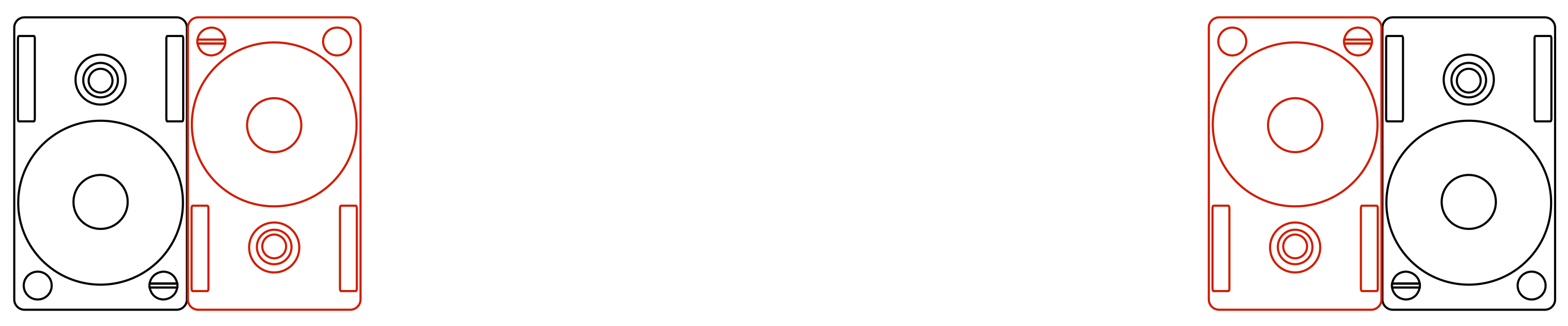
There are advantages and disadvantages of both of these arrangements – but in both cases, there is a lateral shift in the stereo image. When switching between pairs, either you get a left-right shift in image, or a change in width… It turned out that this change was more distracting than the vertical arrangement of the drivers, so we changed configuration to the one shown in Figure 4, below.

Now, instead of switching between loudspeakers, we pretended that one of them was a tweeter and other was a mid-woofer, and switched which was which, on the fly. Our “virtual” crossover was close-ish to the real crossover in the loudspeakers (our crossover was at 3.5 kHz, if you’re curious), so you could say that we were sort-of changing between using the upper tweeter + the lower woofer and using the upper woofer + lower tweeter, the “acoustical centres” of which are roughly at the same height. (remember – this was a quick-n-dirty experiment…)


After having listened to these three configurations of loudspeakers, we decided that the vertical arrangement of the drivers was not important with the vertical separation we were using.
This brought us to the second part of the question… If the tweeter and the midrange were further apart, would we have a preference? So, we kept our virtual crossover, using one loudspeaker as the “tweeter” and the other as the “mid-woofer”, and we moved the loudspeakers further apart, one example of which is shown in Figure 7. (One thing to note here is that when I say “further apart” I’m talking about the separation in the vertical angles of the sources – not necessarily their actual distance from each other. For example, if the loudspeakers were 1 m apart vertically, and you were level with one of the loudspeakers, but the listening position was a kilometre away, then the vertical angular separation (0.057 degrees) would be much smaller than if you were 1 m away (45 degrees)…)

The answer we arrived at at the end was that, when the vertical separation of the drivers gets extreme (perhaps I should use the word “silly” instead), we preferred the configuration where the “mid-woofer” was at ear-height. However, this was basically a choice of which version we disliked less (“preference” is a loaded word…). When the drivers get far enough apart, of course, they no longer “hang together” as a single device without some extra signal processing tricks.
So, we went to lunch having made the decision that, as long as the tweeters and the midranges are close enough to each other vertically, we really didn’t have a preference as to which was on top, so, if anyone asked, we would let the visual designers decide. (Remember that “close enough” is not only determined by this little experiment – it is also determined by the wavelengths of the crossover frequencies and whether or not there are more drivers to consider. For example, in the example in Figure 1, it might be that we don’t care about the relative placement of the tweeter and midrange in isolation – but perhaps putting the tweeter between the midrange and woofer will make them too far apart to have a nice vertical directivity behaviour across the lower crossover…)
This isn’t the first time we asked ourselves such a question. Although I was not yet working at B&O at the time, my colleagues tell me that, back in the days when they were developing the BeoLab 3500 and the BeoLab 7-1 (both of which are “stereo” loudspeakers – essentially two multi-way loudspeakers in a single device) , they questioned the driver arrangement as well. Should the tweeters or the midranges / woofers be on the outside? You can see in the photos of the 3500 on this page that they decided to put the lower-frequency bands wider because the overall impression with stereo signals was wider than if the tweeters were on the outside.
#35 in a series of articles about the technology behind Bang & Olufsen loudspeakers
Take a look at Figure 1. You’ll see a pair of headphones (BeoPlay H6‘s, if you’re curious…) sitting under a lamp that is lighting them directly. (That lamp is the only light source in the room. I can’t prove it, so you’ll have to trust me on this one…) You can see the headphones because the light is shining on them, right? Well… sort of.

What happens if we put something between the lamp and the headphones? Take a look at Figure 2, which was taken with the same camera, the same lens, the same shutter speed, the same F-stop, and the same ISO (in other words, I’m not playing any tricks on you – I promise…).

Notice that you can still see the headphones, even though there is no direct light shining on them. This probably does not come as a surprise, since there is a mirror next to them – so there is enough light bouncing off the mirror to reflect enough light back to the headphones so that we can still see them. In fact, there’s enough light from the mirror that we can see the shadow caused by the reflected lamp (which is also visible in Figure 1, if you’re paying attention…).
If you don’t believe me, look around the room you’re sitting in right now. You can probably see everything in it – even the things that do not have light shining directly on them (for example, the wall behind an open door, or the floor beneath your feet if you lift them a little…)
Exactly the same is true for sound. Let’s turn the lamp into a loudspeaker and the headphones on the floor into you, in the listening position and send a “click” sound (what we geeks call an “impulse”) out of the loudspeaker. What arrives at the listening position? This is illustrated in Figure 3, which is what we call an “impulse response” – how a room responds to an impulse (a click coming from a loudspeaker).

The top plot in Figure 1 shows the signal that is sent to the input of the loudspeaker. The bottom plot is the signal at the input of the microphone placed at the listening room. If we zoom in on the bottom plot, the result is Figure 4. This makes it much easier to see the direct sound and the reflections as separate components.
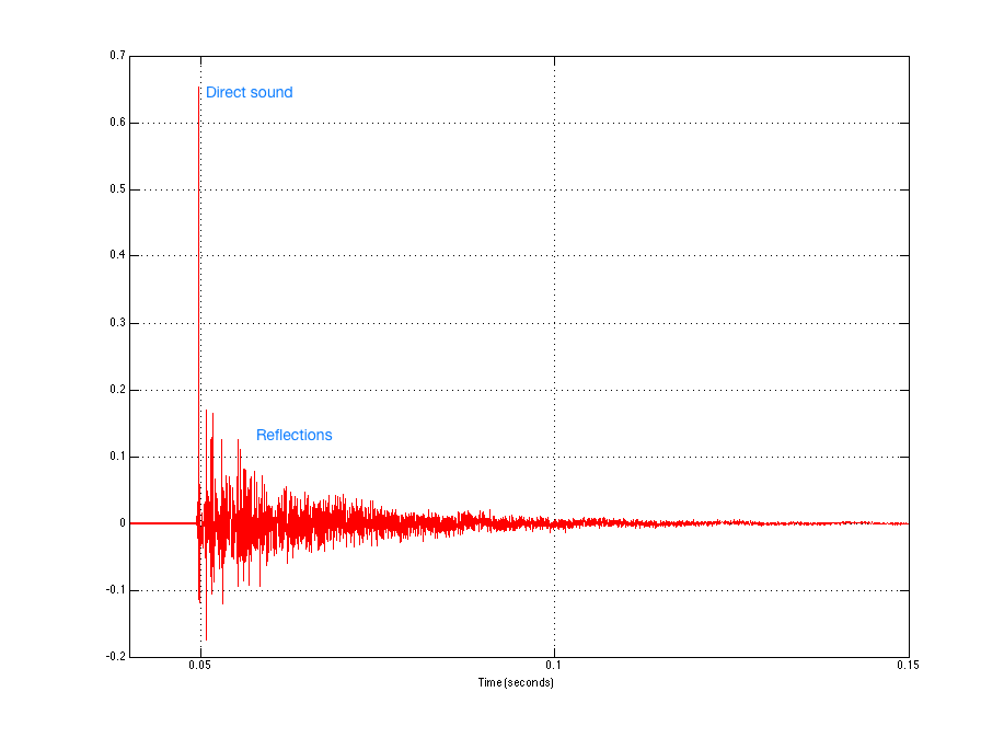
If we zoom in even further to the beginning of the plot in Figure 4, we can see individual reflections in the room’s response, as is shown in Figure 5.

Let’s take the total impulse response and separate the direct sound from the rest. This is shown in Figure 6.

We can then calculate the magnitude responses of the two separate components individually to see what their relative contributions are – shown in Figure 7.

Now, before you get carried away, I have to say up-front that this plot is a little misleading for many reasons – but I’ll only mention two…
The first is that it shows that the direct sound is quieter than the reflected sound in almost all frequency bands, but as you can see in Figure 6, the reflected energy is never actually louder than the direct sound. However, the reflected energy lasts for much longer than the direct sound, which is why the analysis “sees” it as containing more energy – but you don’t hear the decay in the room’s response at the same time when you play a click out of the loudspeaker. Then again, you usually don’t listen to a click – you listen to music, so you’re listening to the end of the room decay on the music that happened a second ago while you’re listening to the middle of the decay on the music that happened a half-second ago while you’re listening to the direct sound of the music that happened just now… So, at any given time, if you’re playing music (assuming that this music was constantly loud – like Metallica, for example…), you’re hearing a lot of energy from the room smearing music from the recent past, compared to the amount of energy in the direct sound which is the most recent thing to come out of the loudspeaker.
The second is in the apparent magnitude response of the direct sound. It appears from the red curve in Figure 7 that this loudspeaker has a response that lacks low frequency energy. This is not actually true – the loudspeaker that I used for this measurement actually has a flat on-axis magnitude response within about 1 dB from well below 20 Hz to well above 20 kHz. However, in order to see that actual response of the loudspeaker, I would have to use a much longer slice of time than the little red spike shown in Figure 6. In other words, the weirdness in the magnitude response is an artefact of the time-slicing of the impulse response. The details of this are complicated, so I won’t bother explaining it in this article – you’ll just have to trust me when I say that that isn’t really the actual response of the loudspeaker in free space…
The “punch line” for all of this is that the room has a significant influence on the perceived sound of the loudspeaker (something I talked about in more detail in this article). The more reflective the surfaces in the room, the more influence it has on the sound. (Also, the more omnidirectional the loudspeaker, the more energy it sends in more directions in the room, which also will mean that the room has more influence on the total sound at the listening position… but there’s more information about that in the article on Beam Width Control.)
So, if the room has a significant influence on the sound of the loudspeaker at the listening position, then it’s smart to want to do something about it. In a best case (and very generally speaking…), we would want to measure the effects that the room has on the overall sound of the loudspeaker and “undo” them. The problem is that we can’t actually undo them without changing the room itself. However, we can make some compensation for some aspects of the effects of the room. For example, one of the obvious things in the blue curve in Figure 7 is that the listening room I did the measurement in has a nasty resonance in the low end (specifically, it’s at about 57 Hz which is the second axial mode for the depth of the room which is about 6 m). It would certainly help the overall sound of the loudspeaker to put in a notch filter at that frequency – in a best case, we should measure the phase response of the room’s resonance and insert a filter that has the opposite phase response. But that’s just the beginning with one mode – there are lots more things to fix…
Almost all Bang & Olufsen loudspeakers have a switch that allows you to change its magnitude response to compensate for the position of the loudspeaker in the room. This is typically called a Free/Wall/Corner switch, since it’s designed to offset the changes to the timbre of the loudspeaker caused by the closest boundaries. There’s a whole article about this effect and how we make a filter to compensate for it at this link.
In 2002, Bang & Olufsen took this a step further when it introduced the BeoLab 5 which included ABC – Automatic Bass Calibration. This was a system that uses a microphone to measure the effects of the listening room’s acoustical behaviour on the sound of the loudspeaker, and then creates a filter that compensates for those effects in the low frequency band. As a simple example, if your room tends to increase the apparent bass level, then the BeoLab 5’s reduce their bass level by the same amount. This system works very well, but it has some drawbacks. Specifically, ABC is designed to improve the response of the loudspeaker averaged over all locations in the room. However this follows the philosophy first stated Spock said in Star Trek II: The Wrath of Kahn when he said “the needs of the many outweigh the needs of the few, or the one.” In other words, in order to make the averaged response of the loudspeaker better in all locations in the room, it could be that the response at one location in the room (say, the “sweet spot” for example…) gets worse (whatever that might mean…). This philosophy behind ABC makes sense in BeoLab 5, since it is designed as a loudspeaker that has a wide horizontal directivity – meaning it is designed as a loudspeaker for “social” listening, not as a loudspeaker for someone with one chair and no friends… Therefore an improved average room response would “win” in importance over an improved sweet spot.
We are currently working on a taking this concept to a new level with Active Room Compensation. Using an external microphone, we can measure the effects of the room’s acoustical behaviour in different zones in the room and subsequently optimise compensation filters for different situations. For example, in order to duplicate the behaviour of BeoLab 5’s ABC, we just need to use the microphone to measure a number of widely-space locations around the room, thus giving us a total average for the space. However, if we want to create a room compensation filter for a single location – the sweet spot, for example – then we can restrict the locations of the microphone measurements to that area within the room. If we want to have a compensation filter that is pretty good for the whole room, but has emphasis on the sweet spot, we just have to make more measurements in the sweet spot than in the rest of the room. The weighting of importance of different locations in the room can be determined by the number of microphone measurements we do in each location. Of course, this isn’s as simple a procedure as pressing one button, as in ABC on the BeoLab 5, but it has the advantage in the ability to create a compensation filter for a specific location instead of for the whole listening space.
As part of this work, we are developing a new concept in acoustical room compensation: multichannel processing. This means that the loudspeakers not only “see” each other as having an effect on the room – but they help each other to control the room’s acoustical influence. So, if you play music in the left loudspeaker only, then some sound will also come out of the right loudspeaker. This is because both the left and right loudspeakers are working together to control the room (which is being “activated” by sound only from the left loudspeaker.
#34 in a series of articles about the technology behind Bang & Olufsen loudspeakers
Go to the middle of a snow-covered frozen lake with a loudspeaker, a chair, and a friend. Sit on the chair, close your eyes and get your friend to place the loudspeaker some distance from you. Keep your eyes closed, play some sounds out of the loudspeaker and try to estimate how far away it is. You will be wrong (unless you’re VERY lucky). Why? It’s because, in real life with real sources in real spaces, distance information (in other words, the information that tells you how far away a sound source is) comes mainly from the relationship between the direct sound and the early reflections that come at you horizontally. If you get the direct sound only, then you get no distance information. Add the early reflections and you can very easily tell how far away it is. If you’re interested in digging into this on a more geeky level, this report is a good starting point.
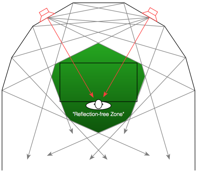
When a recording engineer makes a recording in a well-designed studio, he or she is sitting not only in a carefully-designed acoustical space, but a very special area within that space. In many recording studios, there is an area behind the mixing console where there are no (or at least almost no) reflections from the sidewalls . This is accomplished either by putting acoustically absorptive materials on the walls to soak up the sound so it cannot reflect (as shown in Figure 1), or to angle the walls so that the reflections are directed away from the listening position (as shown in Figure 2).
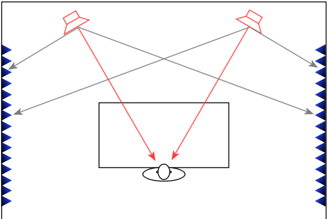
Both of these are significantly different from what happens in a typical domestic listening room (in other words, your living room) where the walls on either side of the listening position are usually acoustically reflective, as is shown in Figure 3.
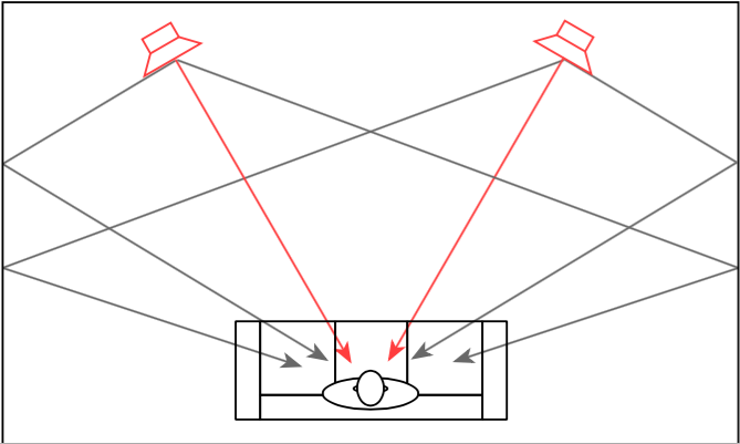
In order to get the same acoustical behaviour at the listening position in your living room that the recording engineer had in the studio, we will have to reduce the amount of energy that is reflected off the side walls. If we do not want to change the room, one way to do this is to change the behaviour of the loudspeaker by focusing the beam of sound so that it stays directed at the listening position, but it sends less sound to the sides, towards the walls, as is shown in Figure 4.
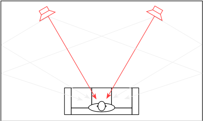
So, if you could reduce the width of the beam of sound directed out the front of the loudspeaker to be narrower to reduce the level of sidewall reflections, you would get a more accurate representation of the sound the recording engineer heard when the recording was made. This is because, although you still have sidewalls that are reflective, there is less energy going towards them that will reflect to the listening position.
However, if you’re sharing your music with friends or family, depending on where people are sitting, the beam may be too narrow to ensure that everyone has the same experience. In this case, it may be desirable to make the loudspeaker’s sound beam wider. Of course, this can be extended to its extreme where the loudspeaker’s beam width is extended to radiate sound in all directions equally. This may be a good setting for cases where you have many people moving around the listening space, as may be the case at a party, for example.
For the past 5 or 6 years, we in the acoustics department at Bang & Olufsen have been working on a loudspeaker technology that allows us to change this radiation pattern using a system we call Beam Width Control. Using lots of DSP power, racks of amplifiers, and loudspeaker drivers, we are able to not only create the beam width that we want (or switch on-the-fly between different beam widths), but we can do so over a wide frequency range. This allows us to listen to the results, and design the directivity pattern of a loudspeaker, just as we currently design its timbral characteristics by sculpting its magnitude response. This means that we can not only decide how a loudspeaker “sounds” – but how it represents the spatial properties of the recording.
Let’s start by taking a simple recording – Susanne Vega singing “Tom’s Diner”. This is a song that consists only of a fairly dryly-recorded voice without any accompanying instruments. If you play this tune over “normal” multi-way loudspeakers, the distance to the voice can (depending on the specifics of the loudspeakers and the listening room’s reflective surfaces) sound a little odd. As I discussed in more detail in this article, different beam widths (or, if you’re a little geeky – “differences in directivity”) at different frequency bands can cause artefacts like Vega’s “t’s” and “‘s’s” appearing to be closer to you than her vowel sounds, as I have tried to represent in Figure 5.
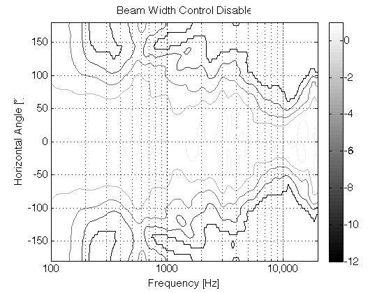
If you then switch to a loudspeaker with a narrow beam width (such as that shown in the directivity plot in Figure 7 – the beam width is the vertical thickness of the shape in the plot – note that it’s wide in the low frequencies and narrowest at 10,000 Hz), you don’t get much energy reflected off the side walls of the listening room. You should also notice that the contour lines are almost parallel, which means that the same beam width doesn’t change as much with frequency.
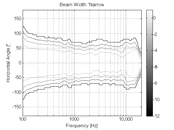
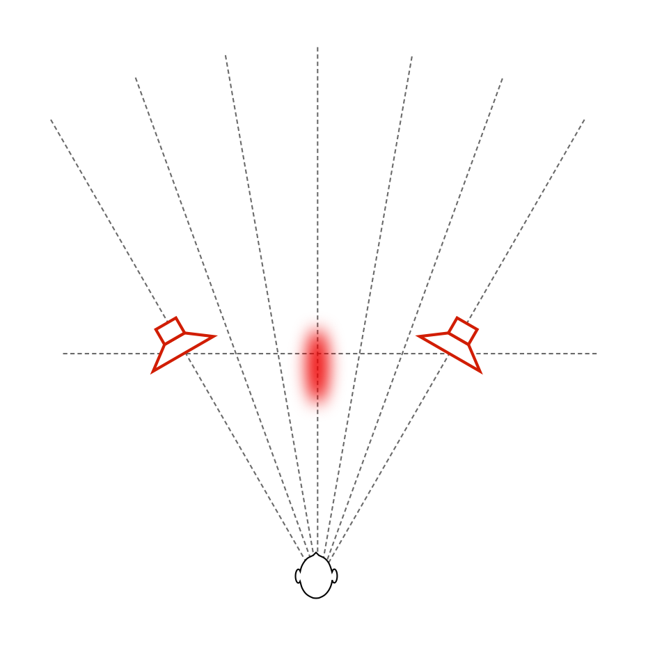
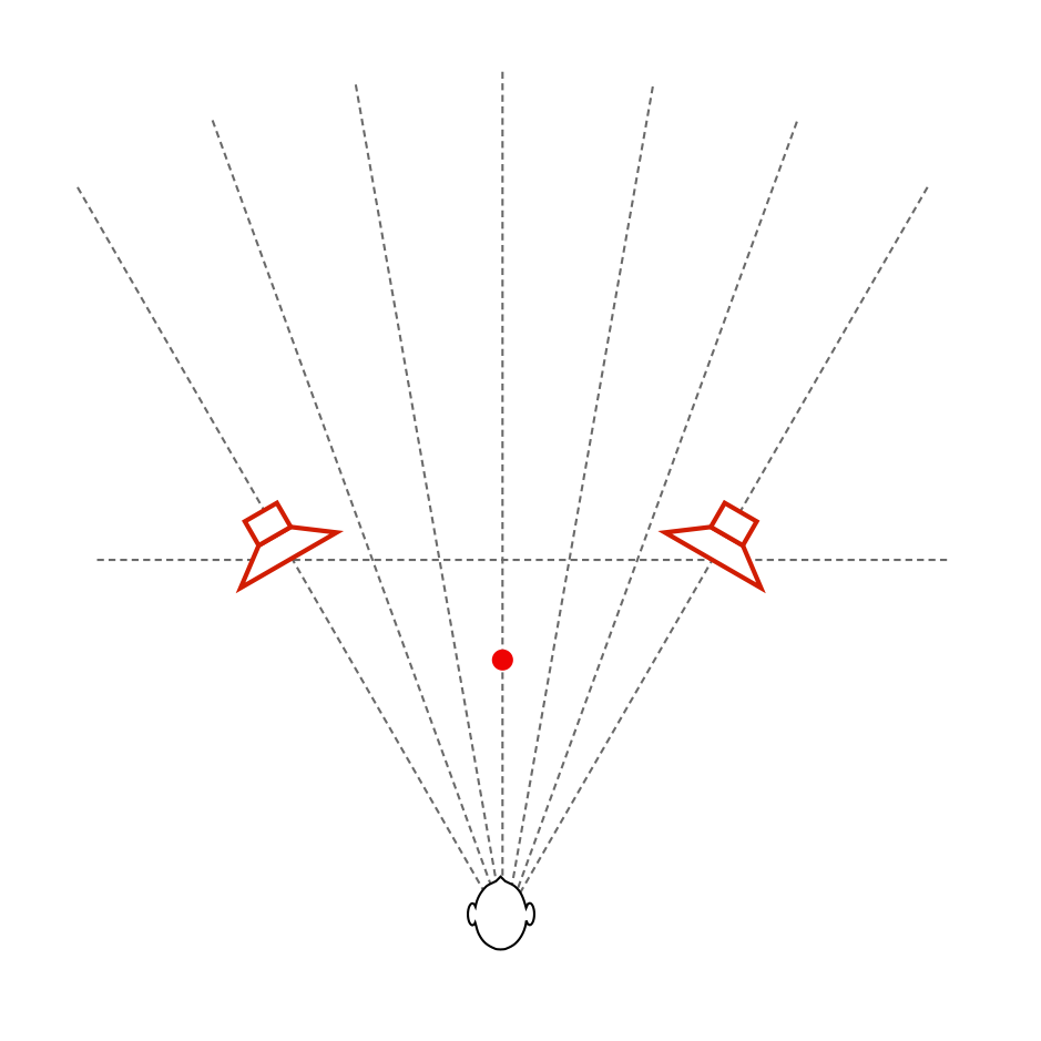
Since there is very little reflected energy in the recording itself, the result is that the voice seems to float in space as a pinpoint, roughly half-way between the listening position and the loudspeakers – much as was the case of the sound of your friend on the snow-covered lake. In addition, as you can see in Figure 7, the beam width of the loudspeaker’s radiation is almost the same at all frequencies – which means that, not only does Vega’s voice float in a location between you and the loudspeakers, but all frequency bands of her voice appear to be the same distance from you. This is represented in Figure 8.
If we then switch to a completely different beam width that sends sound in all directions, making a kind of omnidirectional loudspeaker (with a directivity response as is shown in Figure 9), then there are at least three significant changes in the perceived sound. (If you’re familiar with such plots, you’ll be able to see the “lobing” and diffraction caused by various things, including the hard corners on our MDF loudspeaker enclosures. See this article for more information about this little issue… )
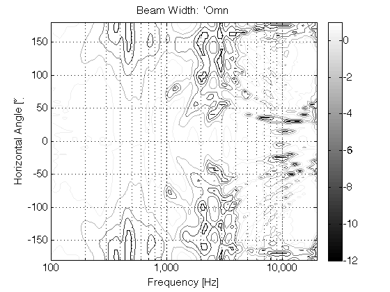
The first big change is that the timbre of the voice is considerably different – particularly in the mid-range (although you could easily argue that this particular recording only has mid-range…). This is caused by the “addition” of reflections from the listening room’s walls at the listening position (since we’re now sending more energy towards the room boundaries). The second change is in the apparent distance to the voice. It now appears to be floating at a distance that is the same as the distance to the loudspeakers from the listening position. (In other words, she moved away from you…). The third change is in the apparent width of the phantom image – it becomes much wider and “fuzzier” – like a slightly wide cloud floating between the loudspeakers (instead of a pin-point location). The total result is represented in Figure 10, below.
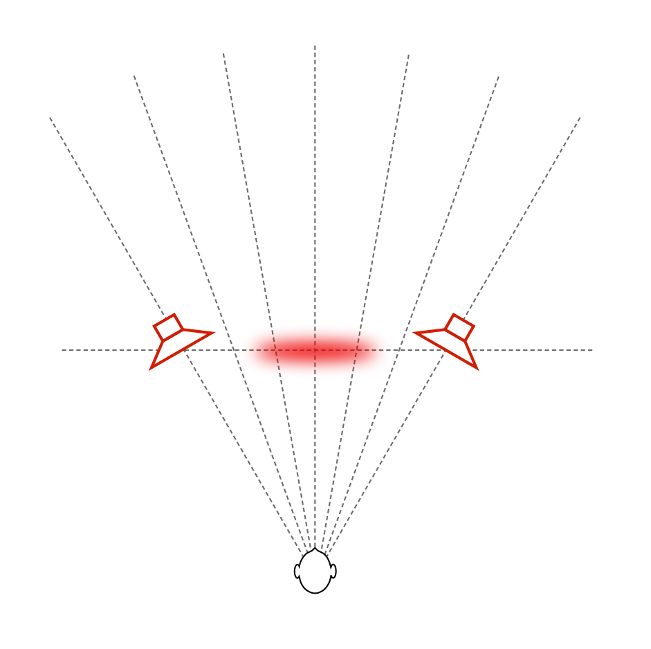
All three of these artefacts are the result of the increased energy from the wall reflections.
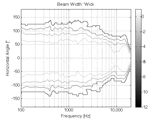
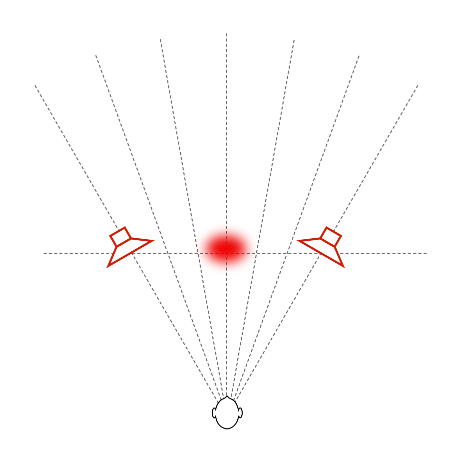
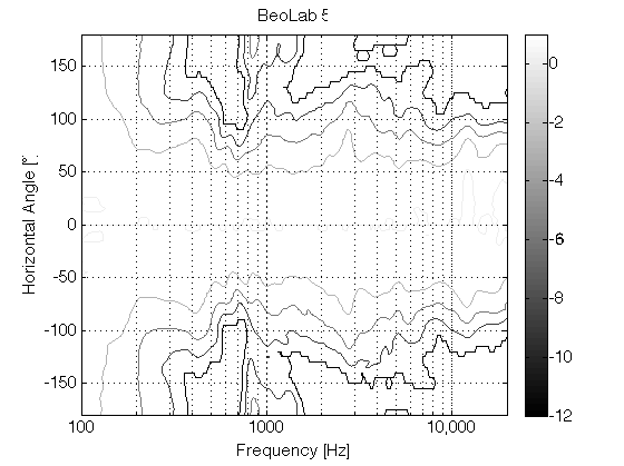
Of course, we don’t need to go from a very narrow to an omnidirectional beam width. We could find a “middle ground” – similar to the 180º beam width of BeoLab 5 and call that “wide”. The result of this is shown in Figures 11 and 12, with a measurement of the BeoLab 5’s directivity shown for comparison in Figure 13.
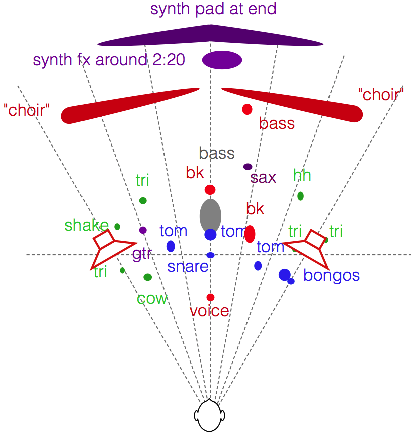
If we do the same comparison using a more complex mix (say, Jennifer Warnes singing “Bird on a Wire” for example) the difference in the spatial representation is something like that which is shown in Figures 14 and 15. (Compare these to the map shown in this article.) Please note that these are merely an “artist’s rendition” of the effect and should not be taken as precise representations of the perceived spatial representation of the mixes. Actual results will certainly vary from listener to listener, room to room, and with changes in loudspeaker placement relative to room boundaries.
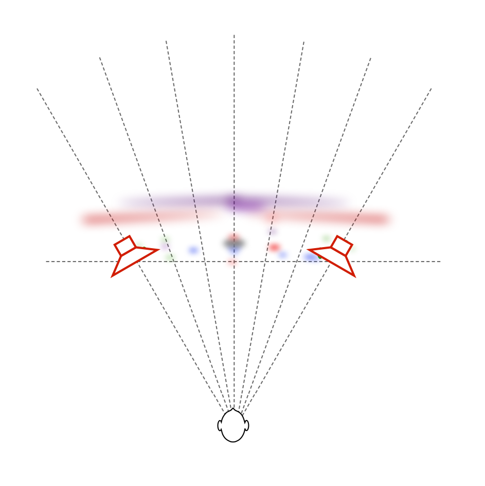
Of course, everything I’ve said above assumes that you’re sitting in the “sweet spot” – a location equidistant to the two loudspeakers at which both loudspeakers are aimed. If you’re not, then the perceived differences between the “narrow” and “omni” beam widths will be very different… This is because you’re sitting outside the narrow beam, so, for starters, the direct sound from the loudspeakers in omni mode will be louder than when they’re in narrow mode. In an extreme case, if you’re in “narrow” mode, with the loudspeaker pointing at the wall instead of the listening position, then the reflection will be louder than the direct sound – but now I’m getting pedantic.
The idea here is that we’re experimenting on building a loudspeaker that can deliver a narrow beam width so that, if you’re like me – the kind of person who has one chair and no friends, and you know what a “stereo sweet spot” is, then you can sit in that chair and hear the same spatial representation that the recording engineer heard in the recording studio (without having to make changes to your living room’s acoustical treatment). However, if you do happen to have some friends visiting, you have the option of switching over to a wider beam width so that everyone shares a more similar experience. It won’t sound as good (whatever that might mean to you…) in the sweet spot, but it might sound better if you’re somewhere else. Similarly, if you take that to an extreme and have a LOT of friends over, you can use the “omni” beam width and get a more even distribution of background music throughout the room.
For more information on Beam Width Control
Shark Fins and the birth of Beam Width Control
For an outsider’s view, please see the following…
“Ny lydteknikk fra Bang & Olufsen” – Lyd & Bilde (Norway)
Stereophile magazine (October 2015, Print edition) did an article on their experiences hearing the prototypes as well.
“BeoLab 90: B&O laver banebrydende højttaler” – Lyd & Bilde (Norway)

A GREAT podcast from 99% Invisible about Tony Schwartz’s recording history and the world’s first “commercial” radio station that started in Frank Conrad’s Garage.
The following posting is a description of a test that I did on two streaming services where I concluded that one of them is probably doing dynamic range compression and the other one probably isn’t.
My conclusion was only partly correct. One of the players was, indeed, doing dynamic range compression. However, this was because I asked it to do so. Since posting this article, I have found an “Advanced Preferences” in the player that includes the option to make the tracks more alike in level. I had this option set to “ON” when I did this test.
So, almost everything you are about to read below is technically correct – but the conclusion that one of the services is “worse” than the other is not fair. I’ll re-do the entire test and re-post the new analysis and conclusions…
My humble apologies….
-geoff
Tom Lehrer once said “Life is like a sewer. What you get out of it depends on what you put into it.” The same is true when you’re testing loudspeakers. What you get out of them depends on what you feed into them.
This is an important thing to keep in mind when you’re listening to loudspeakers. If listen to a pair of loudspeakers for the first time and you decide that there’s something about them that you don’t like, you should make sure that whatever it is that you don’t like about them is not the fault of your source. This might mean that there’s something in the recording that’s causing the issue (like a resonance in the vocal booth, or a clipped master, for example). It might mean that the player has some issues (computer headphone outputs are notoriously noisy, for example). It might mean that you should be careful that you’re not listening to a lower bitrate psychoacoustic CODEC like MP3, for example. Or it might mean something else that isn’t immediately obvious.
This is particularly true if you use a streaming service, of which there seem to be newcomers every day… Now, before we go any further, I’ll warn you that I’m not going to mention any names in this posting. So, don’t email me and ask “Which services were you talking about in that posting? I promise I won’t tell anyone…” There are various reasons for this – just don’t bother asking.
When you choose a streaming service, there are a couple of things to consider. One is the level of service (and therefore, possibly quality) you want to buy. Some services offer better quality for a higher price. Some services offer music streaming for free if you can live with the commercials (typically at the same audio quality as the low-price version). Different services use different CODEC’s. Some use MP3, some use Ogg Vorbis, and some claim to stream lossless signals. You can then choose different bitrates or CODEC’s at different prices.
I’m not going to get into a discussion between the pro’s and con’s of 320 kbps MP3 vs 160 kbps Ogg Vorbis, or whether anything is as “good” as lossless. Lots of people are discussing that on lots of websites. Feel free to go there to have that fight. What I want to talk about is something else: dynamic range compression.
You should beware when you choose a streaming service that some of them apply a dynamic range compression to the music, regardless of the CODEC. This not only means that the quiet tunes are louder, and the louder tunes are quieter. It also means that the quieter sections of the tunes are louder, and the louder sections are quieter. Even worse, in some cases, this my be done on a frequency-dependent basis (using something called a multi-band compressor) which changes the overall spectral balance of the tune over time, and does it differently for different tracks due to their different spectral characteristics.
Since I have no plan to point fingers, my goal here is to help you learn to point your own fingers. In other words, how can you easily find out whether your streaming service is doing more than “just” reducing the bitrate of the audio signal.
The trick to find this out is a simple matter of doing a quick back-to back comparison. I’ll describe the technique assuming that you’re comparing two streaming services using a single computer – but you could (of course) apply this technique to a streaming service vs. local file playback.
For example, open up Player “A” and Player “B” and load “Arlandria” by the Foo Fighters.
Let’s say that, when you go back and forth, the song is quieter in Player A than in Player B (see Figure 1, below, as an example…). This might be for different reasons (like the volume knobs are not aligned, for example…)
Now load “Bird on a Wire” by Jennifer Warnes and play that (which is mastered to have a much lower average (RMS) level than Arlandria – therefore it should be quieter…).
Let’s say that, when you go back and forth, the song is now louder in Player A than in Player B (as is shown in Figure 2). This means that the “volume knob” theory above doesn’t hold (if it did, Player A would always be quieter than Player B).
So, Arlandria is louder in “B” but Bird on a Wire is louder in “A”. This means that at least one (perhaps both) of the two players is doing something with the dynamic range of the tunes. What is most likely is that at least one of the players is making the Foo Fighters too quiet and Jennifer Warnes too loud (relative to their original mastering).
There might be a good reason for this. It could be that Player “A” is designed to be a radio station – good for background music where you press “play” and you never have to chase the signal with the volume control (in other words, you don’t have to suddenly drop the volume during dinner because the Foo Fighters started playing). However, there might be side effects, since it is likely that the dynamic range compression in Player A (assuming for simplicity’s sake that it is only Player A in this example that is mucking around with the levels) is happening on the signal in real-time – and is not based on a gain offset on a per-tune basis (as some software players do…)
So, as you can see, there’s not much of a trick here. It’s just a matter of doing a direct player-to-player comparison, making sure that as many components in the signal path remain constant. (For example, be careful that your computer doesn’t have a compressor on its headphone output if that’s what you’re using. Many computer headphone outputs have some kind of dynamic range stuff happening like noise gating, peak compression / soft clipping or just general envelope shaping.) Best to use a digital output from your computer to a reliable DAC that just does what it’s told, and doesn’t add any fancy effects like volume levelling.
I took two streaming services (each of them delivering their “high quality” option) and routed their outputs to Max/MSP using Soundflower and recorded each as a 16-bit .wav file. Both were set to maximum volume, as was the master volume of my MacBook Pro.
I then used Audacity to manually time-align and trim the files to have exactly the same length (in samples). The length of each file was arbitrary and based more on when the chorus ended than anything else…
For the analyses of peak level (listed in dB FS, even though I know that dB FS is only supposed to be used for RMS measurements… sue me…), total RMS level, and crest factor, I just wrote a small routine in Matlab to look after this for me. The two values shown are for the Left and Right channels for each tune.
I’ve also supplied a screen shot of the entire tracks analysed, shown in Audacity, so you can get an intuitive feel of the difference between the two streaming services.
Some things to look out for here: If the difference in the peak amplitudes matches the difference in the RMS values (and therefore the crest factors match each other) then the differences in the output levels of the two streaming services is the result of a simple change in level for the entire tune – as if someone had changed the volume setting and left it alone for the whole song (this is the technique ostensibly used by at least one ubiquitous computer-based audio player). However, if the crest factors are different for the two streaming services for a given song (meaning that the differences in the peak amplitudes and the RMS values are different from service to service for a given song) then this means that some time-variant dynamic processing is going on – probably something like a compressor, a peak limiter, a soft-clipper, or just a clipper.
Foo Fighters – Arlandia (first 81.67 seconds)
[table]
Streaming Service “A”, Left, Right
Peak Amplitudes (dB FS), -4.2209, -4.1578
RMS (dB FS), -15.6585, -15.2328
Crest factor (dB), 11.4376, 11.0750
[/table]
[table]
Streaming Service “B”, Left, Right
Peak Amplitudes (dB FS), 0.0, 0.0
RMS (dB FS), -7.4978, -7.1929
Crest factor (dB), 7.4978, 7.1929
[/table]

Jennifer Warnes – Bird on a Wire (first 59.43 seconds)
[table]
Streaming Service “A”, Left, Right
Peak Amplitudes (dB FS), 0.0, 0.0
RMS (dB FS), -9.4162, -10.6752
Crest factor (dB), 9.4162, 10.6752
[/table]
[table]
Streaming Service “B”, Left, Right
Peak Amplitudes (dB FS), -0.1287, -0.3205
RMS (dB FS), -16.5152, -17.8888
Crest factor (dB), 16.3865, 17.5683
[/table]

Lorde – Royals (first 73.46 seconds)
[table]
Streaming Service “A”, Left, Right
Peak Amplitudes (dB FS), -0.0863, -0.0863
RMS (dB FS), -11.0863, -11.0712
Crest factor (dB), 11.0000, 10.9849
[/table]
[table]
Streaming Service “B”, Left, Right
Peak Amplitudes (dB FS), -0.0005, -0.0005
RMS (dB FS), -11.0509, -11.0365
Crest factor (dB), 11.0504, 11.0360
[/table]


So, what confuses me at the end of this is that Royals is almost identical in both. And, before you jump to conclusions, I checked… I did not screw up the captures. When I subtract “B” from “A”, I can hear artefacts typical of a psychoacoustic CODEC, so I know that the two are different enough to be measurably different. What doesn’t make sense is that, if “A” is dynamically compressing the other two tracks more than “B” (which it appears to be), then why is it not messing around with “Royals”? Hmmmm… I guess that more investigation is necessary with respect to this little anomaly – but not today… Sorry.
We can also check to see if the dynamic range compression that’s being used is a multi-band type or not by doing a quick spectral analysis of the excerpts. I took each of the 6 files (three songs x 2 streaming services) and did the following:
Now, before you start complaining about my methodology here, remember that I’m just using a “big paint brush” approach to checking this out. I’m just interested in seeing if there are any significant differences between the spectral balances of a single track coming from the two streaming services. The results are plotted below.


What you can see in those three plots is that the spectra of a given tune from the two services are roughly the same – only the overall levels are different (which roughly correspond to the RMS values shown in Figure 4).
In case you’re curious, if you level-align the plots in Figures 5 through 7 inclusive, you’ll see that the worst-case differences in spectra for the three tunes across the entire frequency range analysed are about 0.7 dB for Arlandria, 0.9 dB for Bird on a Wire, and 0.08 dB for Royals. However, be a little careful here, since this is an RMS value of the entire track – and may not reflect the more “instantaneous” spectral differences, say, on a clipped peak in “Bird on a Wire”, for example. I won’t bother to analyse those, since it would not be surprising for a peak compressor to generate distortion-like harmonics when it’s changing its gain. This could result in a spectral difference that looks like a multi-band compressor, but isn’t. Windowing can be distracting sometimes…
One moral of the story here is that knowing the psychoacoustic CODEC and bitrate used by your streaming service is not necessarily enough information to know whether or not you’re getting the audio quality you may want.
The other moral is that you shouldn’t necessarily trust that a “high quality” version of a streaming service is the same as the “high quality” version of another streaming service.
Another message here is that you should not compare one service to another one and think that you’re only comparing CODEC’s – for example, don’t listen to Deezer vs. Spotify vs. Tidal in order to find out if you can hear the difference between MP3, Ogg Vorbis, and lossless. You might hear a difference, but it might not be caused by the CODEC’s…
Finally, an important moral is: if you’re using a streaming service to test loudspeakers (for example, in a store) – make sure that the version of the tune that you’re listening to is the version that you know – from the same streaming service and the same quality level. Otherwise, the problems (or just differences) you might hear might not be the fault of the speaker… (For example, if your streaming service at home is “worse” than the store’s – it might make the speakers sound better then you think just because the source is better…) Remember garbage in = garbage out, regardless of whether the description is more applicable to the loudspeakers at the store or the ones at home.
I thought it might be interesting to compare a CD version to the streaming versions. Unfortunately, the only disc I have of the three tracks here is the Foo Fighters. I have the original Famous Blue Raincoat album from once-upon-a-time, but I don’t have the 20th anniversary re-release, which is what the streaming services appear to be using.
[table]
Streaming Service “A”, Left, Right
Peak Amplitudes (dB FS), -4.2209, -4.1578
RMS (dB FS), -15.6585, -15.2328
Crest factor (dB), 11.4376, 11.0750
[/table]
[table]
Streaming Service “B”, Left, Right
Peak Amplitudes (dB FS), 0.0, 0.0
RMS (dB FS), -7.4978, -7.1929
Crest factor (dB), 7.4978, 7.1929
[/table]
[table]
Ripped from CD, Left, Right
Peak Amplitudes (dB FS), -0.0003, -0.0003
RMS (dB FS), -10.7888, -10.3700
Crest factor (dB), 10.7885, 10.3697
[/table]
So, the data shows that, at least for this tune, the version ripped from a CD is different again from the two streaming services. This can also be seen if we put the three versions side-by-side on a DAW.

As can be seen below, this means that some samples are clipped in the process in the streaming service that are not clipped in the original…
