This posting is just wrapping up the series. No more plots… I promise.

Of course, this entire series has focused the “greatest hits” of the crossover club which is a limited number of crossover types. There are many other options that I haven’t talked about, but my point was not to explain how to choose and design a crossover for a loudspeaker for the DIY’er. It was to

• give a primer on some of the things to consider when implementing a crossover
• instil instinctive suspicion and doubt when you read an advertisement (or a comment on the Internet) that says something like “this loudspeaker is good (or bad) because it has THIS kind of crossover.”

There are plenty of things that I didn’t (and won’t) talk about, such as:

• Crossovers for loudspeakers with more than two outputs
• Other crossover designs. For example, as a start, search for:
  • Malcom Hawksford Asymmetrical Crossover
  • Malcom Hawksford discussion of stochastic crossovers associated with DMLs
  • Linkwitz’s page on crossover design
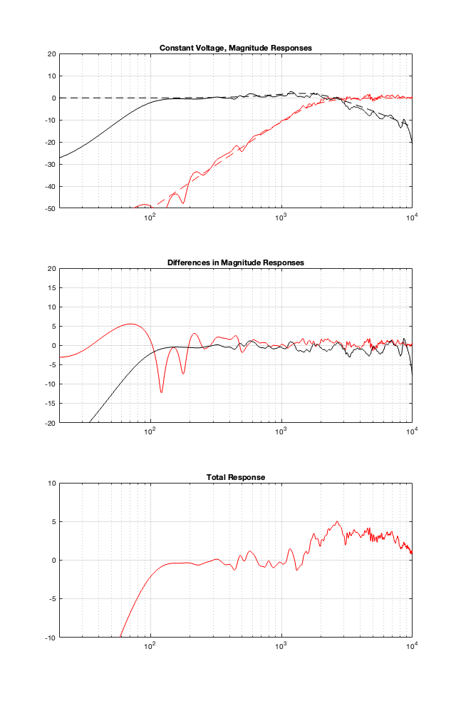
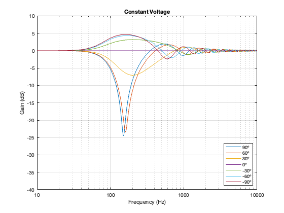
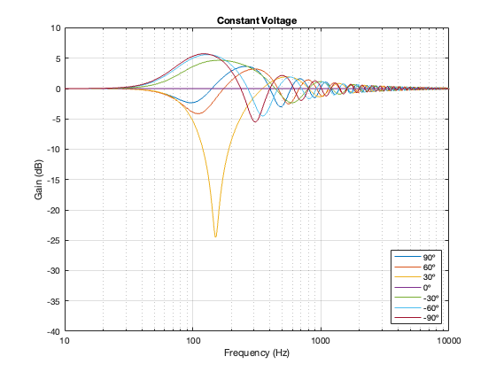
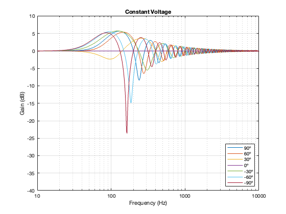
  • “Constant-Voltage Crossover Network Design” by Richard Small

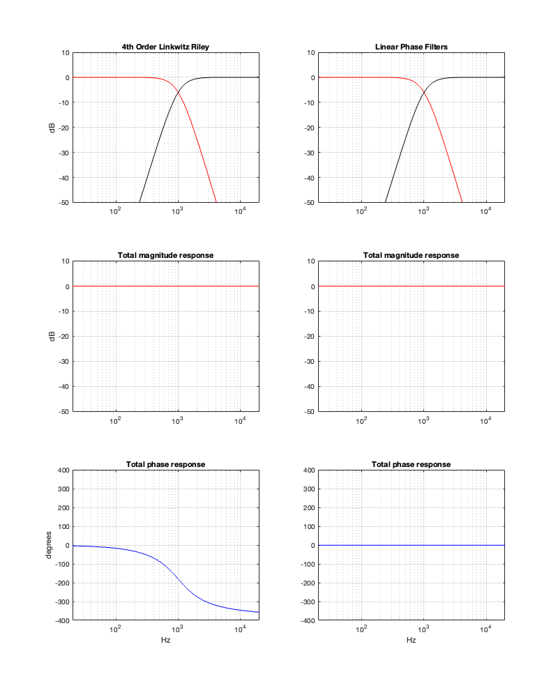
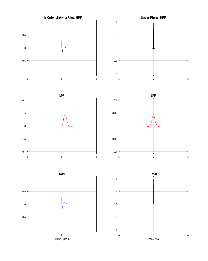
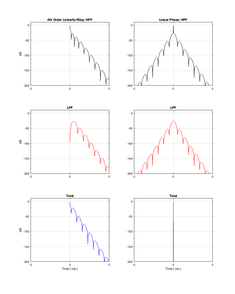
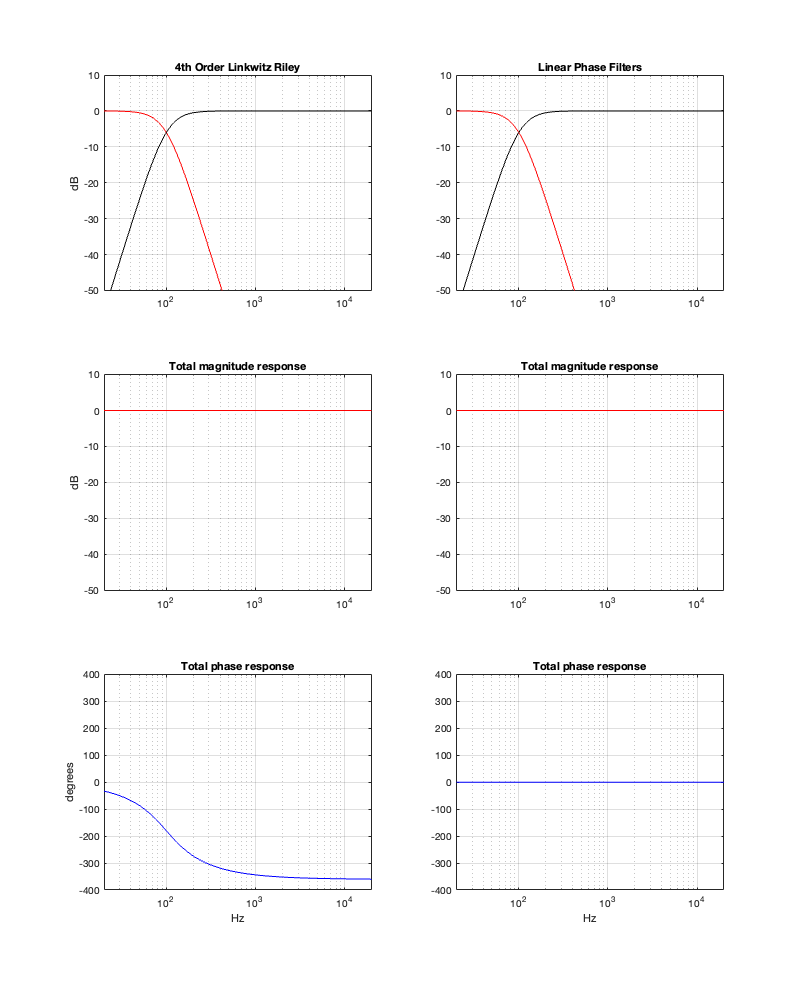
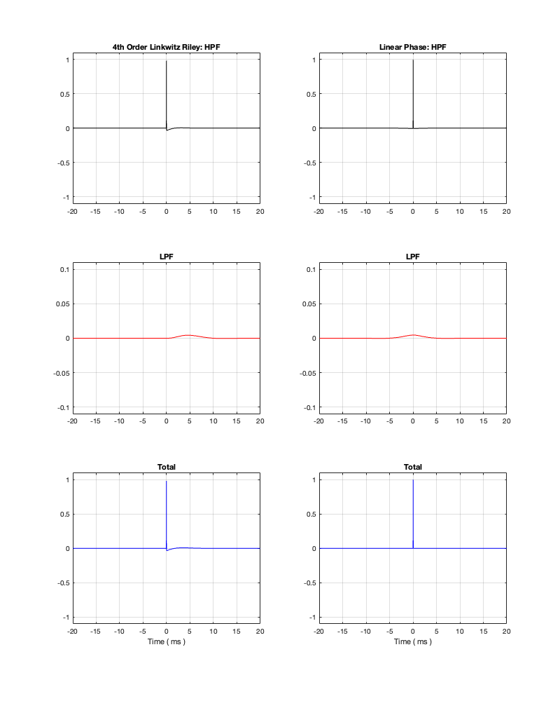
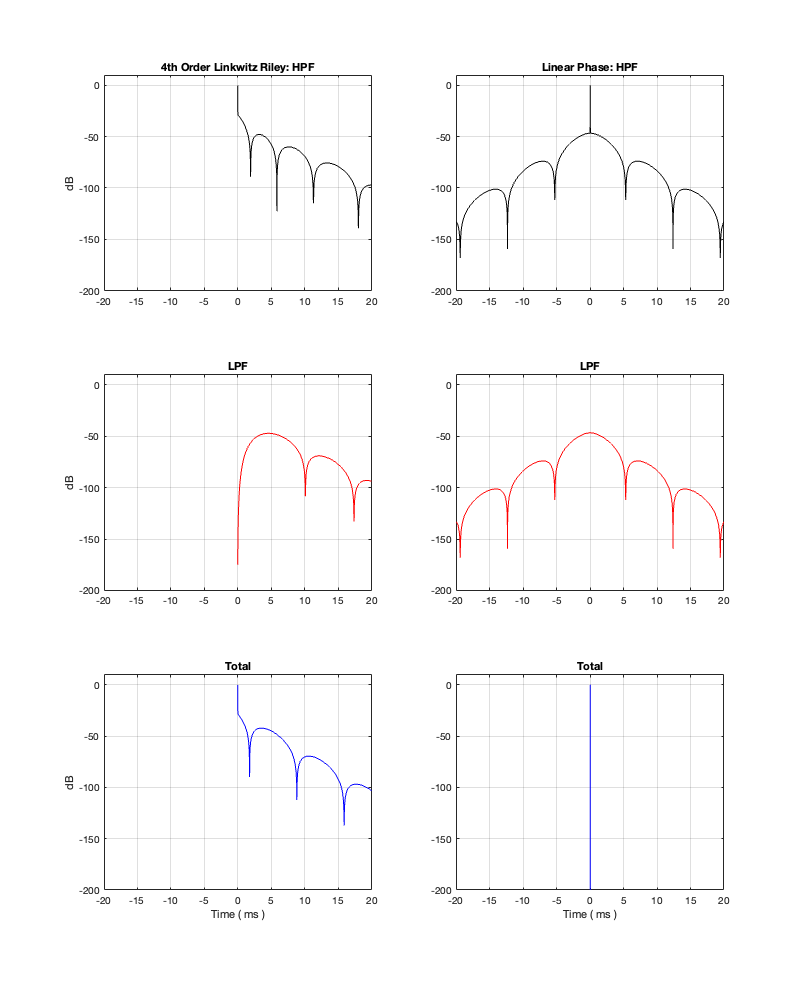
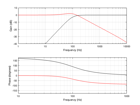
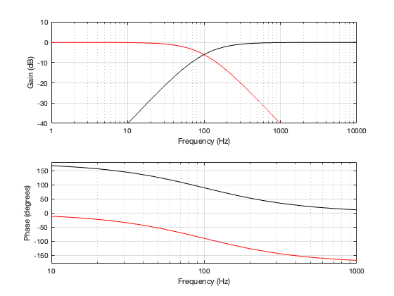
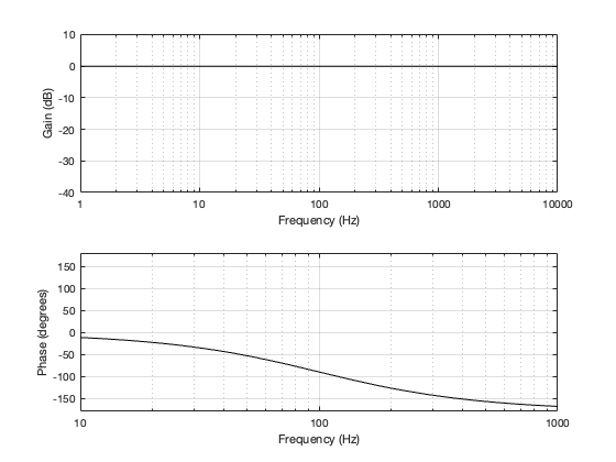
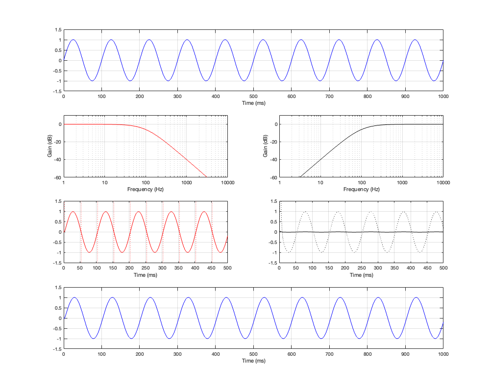
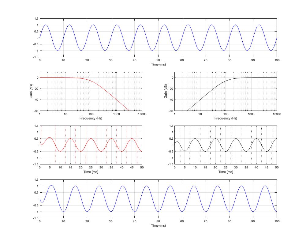
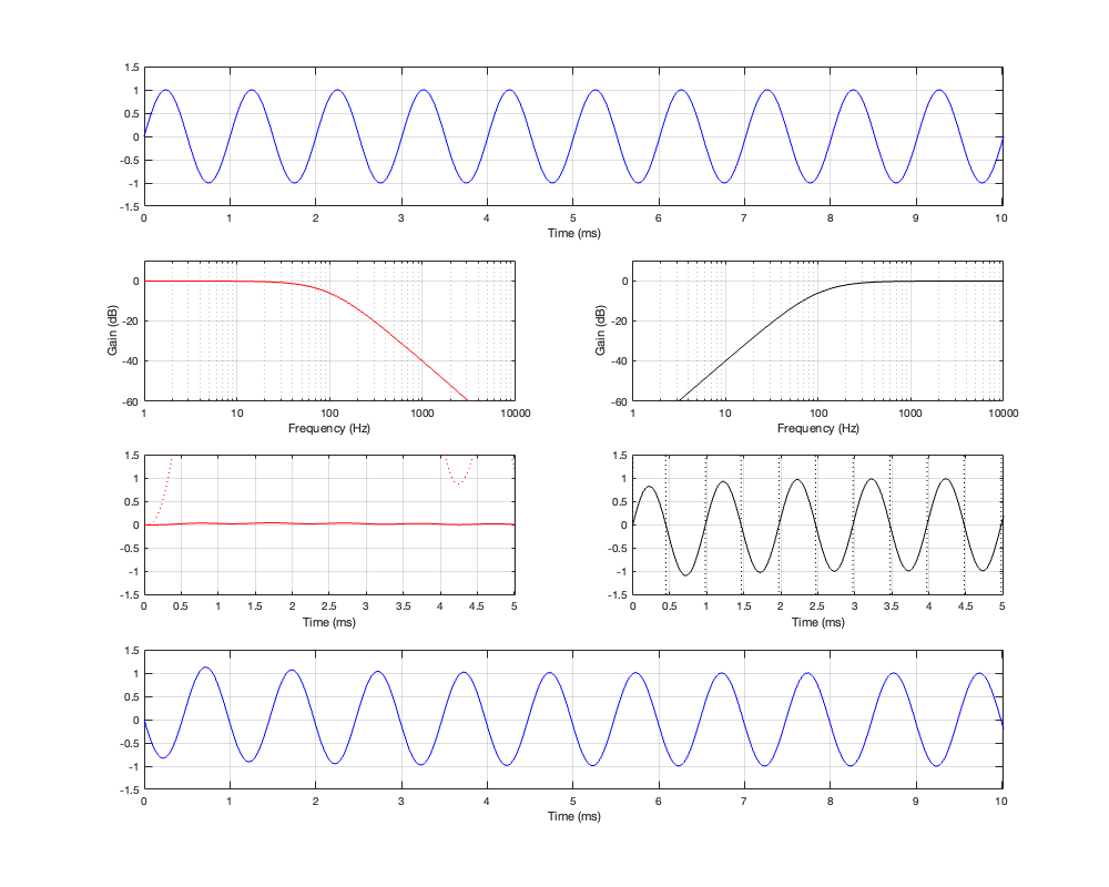
On thing that I intentionally avoided was crossover designs that use filters with extremely high orders, sometimes called “brick wall” crossovers. On paper, they avoid the possible issues with a signal in a given frequency band coming from two sources (e.g. a woofer and a tweeter), so if you ONLY consider them from this perspective, they’re a good idea. However, in my opinion, this is outweighed by the facts that you will probably get a discontinuity in the power response (unless the two drivers have identical three-dimensional radiation patterns at the crossover frequency) AND you will probably have a complete mess in the time domain. Bonkers-order filters aren’t free. (If you clicked on the link to Linkwitz’s page, above and just taken a quick glance, then you’ve probably read the statement at the top of the page that says “The sum of acoustic lowpass and highpass outputs must have allpass behavior without high Q peaks in the group delay.” One way to look at the group delay of a filter is to look at the slope of the phase response. If you make a crossover with really high-order filters, then one of the artefacts will be a high slope in the phase response around the crossover frequency.)

One other thing that I have not mentioned is the incorrect naming that is often associated with crossovers and filters in general. Many people say “FIR Filter” (Finite Impulse Response) when they actually mean “Linear phase filter”. It’s important to remember that you can’t have a linear phase filter without an FIR filter implementation, but certainly not all FIR filters are linear phase. (Weirdly, a linear phase filter does, in fact, have an infinite impulse response, both forwards and backwards in time… But that’s a description of the filter’s response and not how it would be implemented in a DSP-based signal flow.) This incorrect usage drives me nuts. (Then again, many things like this do. For example, I get annoyed when HR people draw a triangle on a whiteboard and call it a pyramid. You never know what’s going to set me off on a pedantic rant about nomenclature.)

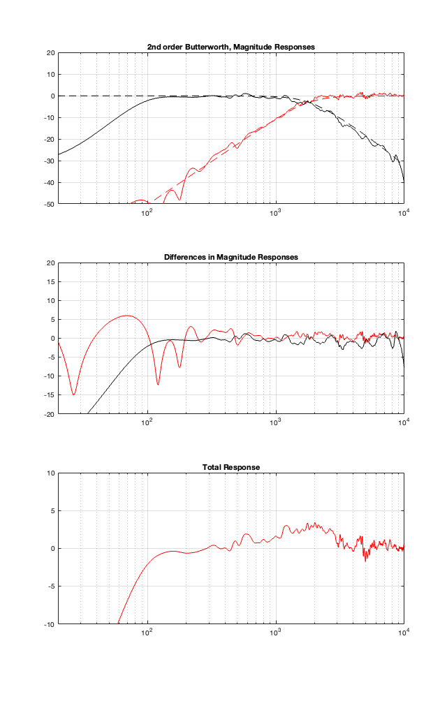
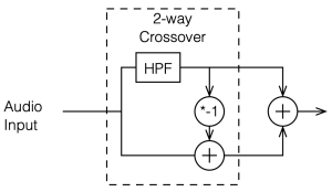
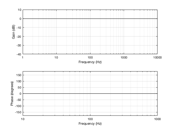
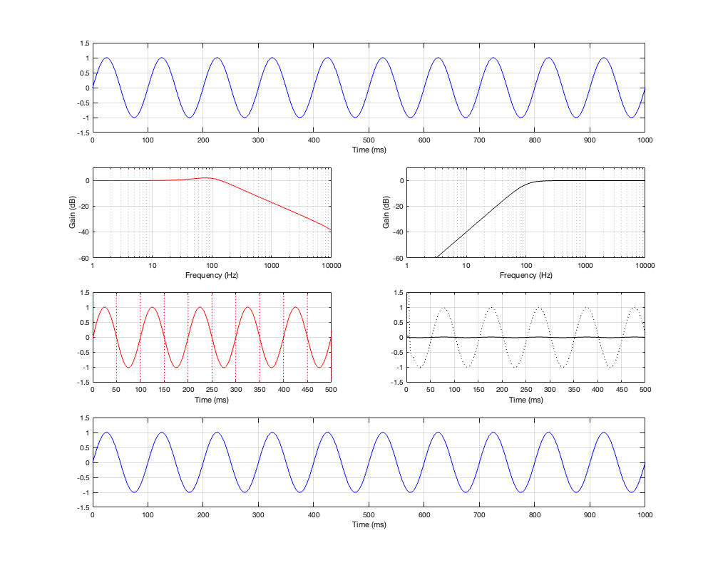
The other thing that I didn’t talk about was another way to look at a Butterworth two-way crossover, in which you see it as lacking a component in the s-domain (using Laplace analysis), which is the reason its sum has an allpass characteristic. If you add the missing component (for example, using a third loudspeaker driver), then the allpass behaviour disappears. This is the concept behind Bang & OIufsen’s “Uni-phase” series of loudspeakers in the 1970s and 1980s. If you want to learn more about this, I’ve already written about it here, and Erik Bækgaard’s original paper from 1977 describing the idea more fully can be found here.

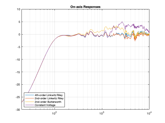
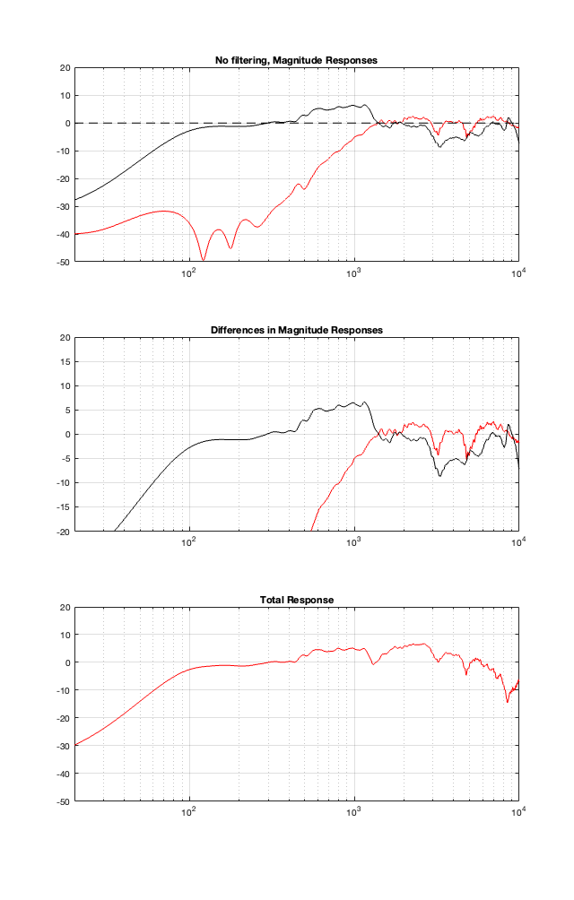
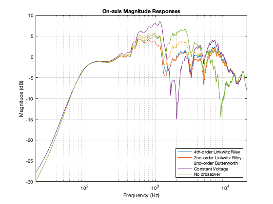
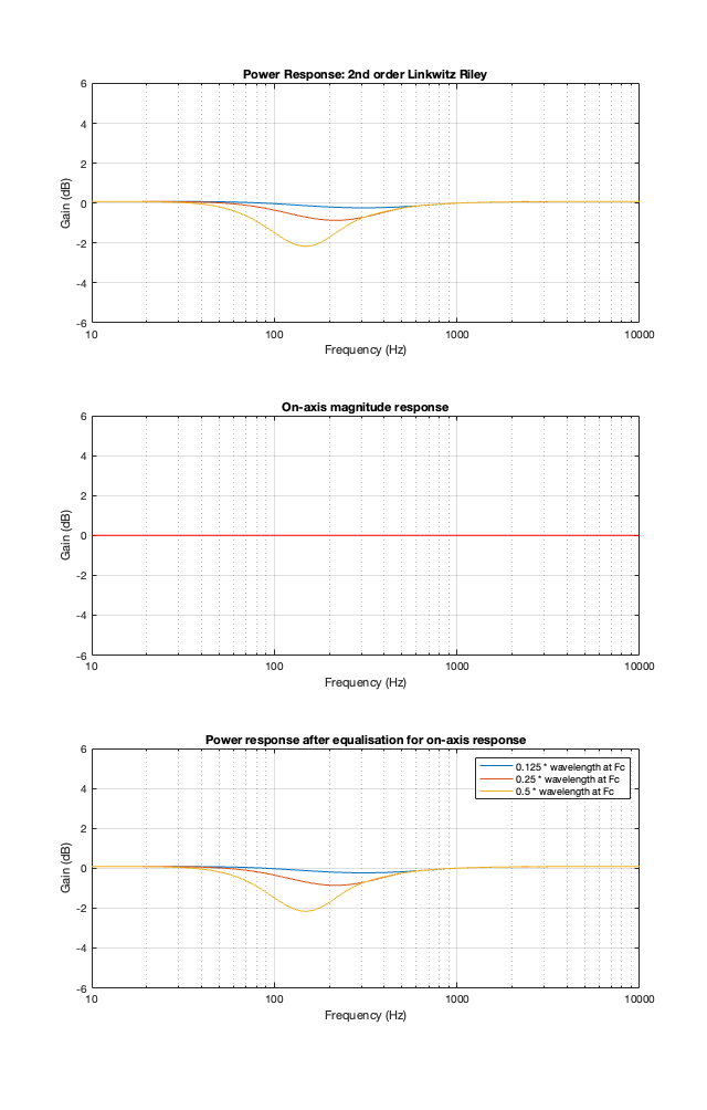
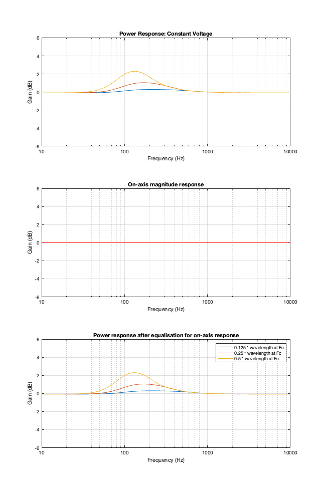
Finally, hopefully, you won’t come away from all of this with a conclusion that one crossover is the winner. A crossover is just one component in a long series- and parallel-chain of components that make up a loudspeaker. Changing any of the other components may require making a different decision about another. And, in order to make that decision, you can’t just consider the on-axis response (unless you live alone in an anechoic chamber (or outdoors…). You also need to think about things like

• the off-axis responses
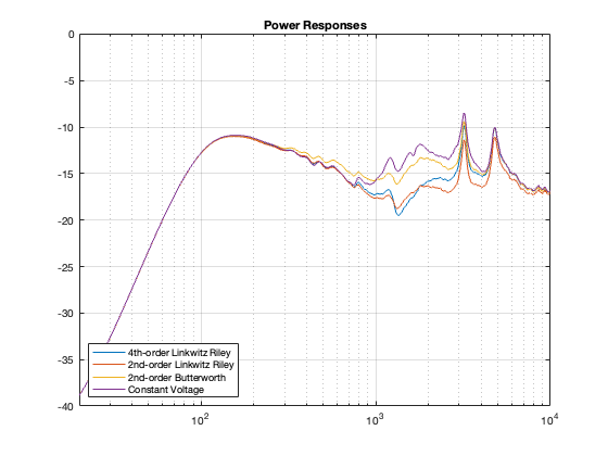
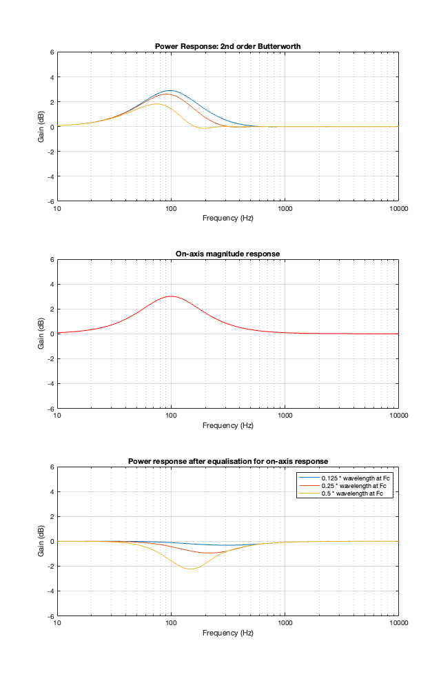
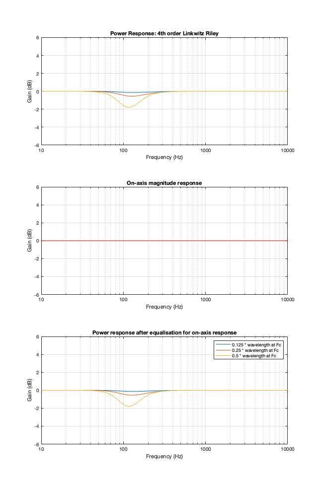
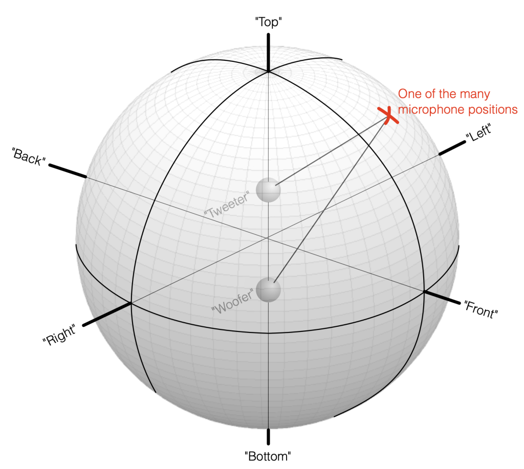
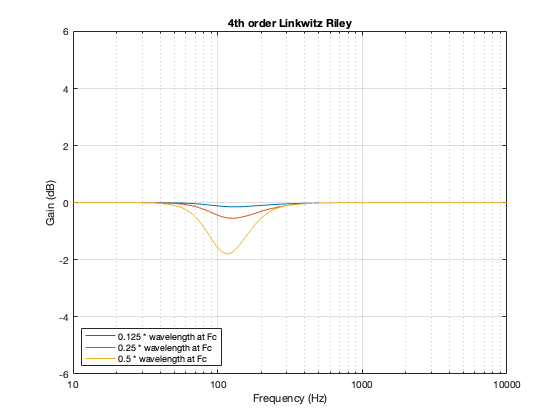
• the power response
• the phase response
• the time response
  and maybe also
• the implications on latency
• your required signal processing power (e.g. in MIPS)
• maybe some other stuff if you have checked all those boxes.

On the other hand, after all this, you should also know that you can’t just implement a crossover ignoring everything else in the chain, and think that it’ll just work. It won’t.

Up to now in this series, we’ve looked at 4 different types of crossover designs:

• 4th-order Linkwitz Riley
• 2nd-order Linkwitz Riley
• 2nd-order Butterworth
• One version of a Constant Voltage design

These have been interesting because they’re popular designs, and they are implementable using either analogue circuitry or digital signal processing (DSP). So, everything I’ve said so far is independent of whether the processing is analogue or digital. This is even true of all of those equalisers I applied to the two loudspeaker drivers to force them to be flat. Those are easiest to implement with DSP, but I didn’t do anything there that can’t be done with resistors, capacitors, and inductors.

But, the original question was

In passive crossovers, many are phase incoherent, 
meaning that the phase shift of one frequency will be different than another frequency. 
Do you agree?  Am curious how this is dealt with in the active crossover’s of B&O products?

Hopefully, it’s obvious that the answer to the first question is “yes” – sort of… Passive crossovers are not “phase incoherent” – but they do have an effect on the phase response. As I’ve shown, you can think of the end result of a crossover implemented with minimum phase filters as an allpass filter. So there is an effect on the phase response of the loudspeaker. (Yes, the on-axis response of a Constant Phase crossover can result in a flat phase response, so that one might be an exception.)

However, if we leave analogue signal processing behind and go forwards limited to digital signal processing, then we have another option: linear phase filters.

To start, let’s look at our original, simplified method of analysing a crossover, using the block diagrams shown in figures 12.1 and 12.2

If we use this signal flow and create two crossovers at 1 kHz, one with a 4th-order Linkwitz Riley design (which I’ve already shown) and one with linear phase filters, the responses will look like the ones shown below in Figure 12.3

Looking at the magnitude responses, you can see that these two filter designs are identical. However, the phase responses of their total outputs are not. The Linkwitz Riley design behaves like a minimum phase allpass filter, whereas the linear phase design does not.

So, this proves that a linear phase crossover is better, right? Not so fast… We’re not done yet…

Time response

The plots above show the frequency responses (“frequency response” is the combination of the magnitude response and the phase response) of the two designs. However, there is another way to look at the response of a system like a crossover, and that is to analyse how it behaves in time.

If we create a signal that is complete silence, and then a single one-sample-long “click”, we have something called an “impulse”. If we then send that into an audio system (like a crossover, for example), then we can see how it behaves in time – its temporal response. Since this method shows us how the system responds when you send an impulse through it, we call it the “impulse response” of the system.

If we measure the impulse responses of our two 1 kHz crossovers, we get the results shown below in Figure 12.4.

As can be seen in the impulse response plots for the Linkwitz Riley crossover, until the impulse arrives at the input of the filter, the output of the filters are silence. This is the flat line with a constant amplitude of 0 from -5 ms to 0 ms. Then, at time = 0 ms, the impulse hits the input of the crossover, and something happens. The output of the high-pass filter spikes, and the output of the low-pass filter slowly (relatively speaking) starts ramping up. The combined output of the two filters, shown in blue, shows that the output is not a single-sample impulse. It has the characteristic shape of the impulse response of an all-pass filter.

The impulse responses of the high-pass and low-pass outputs of the linear phase crossover are similar-ish… but they have one characteristic that is VERY different. They have an output on the left side of time = 0 ms. One way to look at this is to say that they output a signal before the crossover gets something at its input. This is, of course, impossible: linear phase filters are not time machines.

So, how does this happen? By including a delay in the signal flow. In order to make a linear phase filter, you have to include a delay that starts is as long as is necessary to look after the stuff that you need to do to the signal before that big spike hits. So, if you want to use a linear-phase filter, then the “price” is that the output is going to be late.

How late? That’s up to you, since it’s a combination of the filter’s frequency and how accurate and precise you want the filter to be. One way to consider this is to look at the plots in Figure 12.4 on a decibel scale. This is shown in Figure 12.5.

Let’s say, for example, that you have this crossover at 1 kHz and you want to have an impulse response that is accurate down to -100 dB. Looking at HPF and LPF impulse responses for the linear phase crossover, we can see that they drop below -100 dB at about ± 2.4 ms. This means that, if you decide that your threshold of acceptability is about -100 dB (which is pretty good…) then, for a 1 kHz linear phase crossover, you’ll have to include a 2.4 ms delay in your signal path to implement it.

Of course, if you are more picky – say, you want to go down to -200 dB instead, then you’ll have to wait about 4.8 ms (check where the red and black lines get 200 dB down on the left side of the plots.

Notice that I said above that this amount of time – the delay (or as we normally call it: the loudspeakers input-output latency) is also dependent on the frequency of the filters.

So, let’s look at the same plots for a crossover that is one decade lower: at 100 Hz.

Figures 12.6 to 12.8 show the same plots for at 100 Hz crossover. HOWEVER: notice that the scale of the x-axis has changed to ±20 ms instead of ±5 ms. Also note that, despite me extending that scale by a factor of 4, it’s still not enough to get down 200 dB for the linear phase filters.

You can see there (looking at the red curve on the right of Figure 12.8) that, if you’re going to set -100 dB as your threshold, then you will have to have a latency of about 14 or 15 ms to implement it as a linear phase crossover. (Similar to the 1 kHz version, if you want to go down 200 dB, you’ll need to double this to 28 to 30 ms, which is starting to get close to the acceptable limits for lip-synch with video.)

In the next posting, we’ll look what happens to the magnitude and phase responses if you shorten these impulse responses using a technique called “windowing”.

However, I am NOT going to talk about audibility of a linear phase vs a minimum phase strategy. There are people who love to bang on about ringing and pre-ringing and whether you can hear the “ramp in” of the linear phase filters, or whether the “long” decay time of the minimum phase filters are audible. The best way to stay out of this fight is to not comment on it. If you want to decide whether you can hear these things or not, then you should implement them and have a listen. I can’t tell you what you can or cannot hear. However, if you DO decide to try implementing these for a listening test, make sure that you do it right, that:

• the only difference in the crossovers is what you think it is (If not, you’re not comparing the crossover types in isolation), and
• you are running a blind test (if not you can’t trust your own opinion).

In this posting, we’ll do something similar to the analyses from Part 7. In that one, we

• took two point-source theoretically perfect loudspeaker drivers (which means that they have the same magnitude response in all directions in 3D space), (pretending that they were a tweeter and a woofer in a non-existent cabinet)
• filtered each of their inputs using a crossover network
• separated them by some distance
• measured them in a bunch of places on a sphere surrounding the non-existent cabinet
• found the total magnitude response of the system when measured all around on that sphere, which is called the loudspeaker’s Power Response.

Now, we do that again, but we will include the real loudspeaker drivers’ measurements in that three-dimensional world. In this case, we still have the 1″ tweeter and the 6″ woofer in a sealed cabinet. Those two loudspeaker drivers were individually measured at 130 points around them on that sphere that I showed in Part 7.

I then take each of those 130 measurements for each driver, filter them using the crossover, and add the two outputs together, which gives me the magnitude response of the entire loudspeaker with two drivers for each individual location. We then add the 130 measurements to find a total combined response which is the Power Response of the two-way loudspeaker with two real loudspeaker drivers in a real cabinet, with the 5 different crossover types that we’ve been talking about.

Note that I have NOT done what I said I SHOULD do at the end of part 9. I have just been dumb and stuck the crossovers in front of the loudspeaker drivers without thinking about modifying the filters to compensate for the drivers’ characteristics.

The five resulting power responses are shown in Figure 10.1.

The first thing to notice is that there is a roll-off in the low end. This is the natural response of the woofer that we saw in Part 9.

The second thing that you’ll notice is the general downward-slope in the top octave of the plot, starting at about 7 kHz and having a generally decreasing magnitude the higher you go in frequency. This is the result of “beaming”. Since the two loudspeaker drivers, generally, have less and less high-frequency output as you move off-axis, then this appears as less total output from the system on that sphere. If the two loudspeakers were omnidirectional, then the power response would be a horizontal line. The more directional the drivers, the steeper the downward slope of this plot.

The last thing that’s easy to see in this plot is the transition between the woofer and the tweeter. It appears as that steep slope just above 1 kHz. Remember that I put the crossover at 1.8 kHz – so the slope doesn’t sit right on the crossover frequency. But it’s easy to see that something is happening to the directivity of the loudspeaker in that area.

Now remember back to Part 7, where we did a little trick where we made an assumption that a person building or installing a loudspeaker would measured its on-axis response, and then put in an equaliser to flatten this measured response.

In the old days, you would do this “by eye” using something like a graphic or a parametric equaliser. But nowadays, we have fancy tools that can do measurements and create complicated FIR filters that do whatever we want. This means that we can REALLY screw things up with the precision of a surgical scalpel…

So, let’s be dumb and do the same thing again. We’ll take the on-axis responses of the loudspeaker with the different crossovers (we already saw these in Part 9, but here they are again, shown in Figure 10.2), and we’ll make five “perfect” equalisers that make each of these five responses perfectly flat.

After applying each of these customised filters that make our on-axis measurement look like a laser beam, we should probably check what happened to the power responses. They’re shown below in Figure 10.3.

As you can see there, the low frequency response flattens out. This is because we’re really boosting the bass (to fix the on-axis measurement) and this loudspeaker happens to be fairly omnidirectional below about 200 Hz.

You can also see that I was REALLY dumb when I made those equalisation filters. For example, the notch in the on-axis response of the Constant Voltage caused me to make a horrendous peak that results in a really nice-looking plot at one on-axis point in space, but completely messes up the response of the loudspeaker in almost all other directions, resulting in that giant 15 dB peak around 2 kHz (remember that our crossover frequency is in this region…). I also wound up pushing up the low end by something like 30 dB, which is nuts.

The moral of this story is “don’t fix the on-axis response without considering the power response”. OR “just because it looks flat doesn’t mean that it’ll sound good.” On the other hand, notice that, after equalisation, most of the other curves look pretty similar-ish which means that maybe doing some intelligent equalisation for the on-axis response isn’t necessarily a bad idea.

Remember, however, that we’re still only looking at the loudspeaker in infinite space. There’s no room “singing along” with this loudspeaker… but the topic of room compensation is for another time…

N.B. About a week after I made this posting, I found an error in my Matlab code that calculated the plots. They’ve now been updated to the correct curves. The conclusions listed in the text haven’t changed, but some of the little details have.

Extra note for the sake of transparency

Figure 10.3 was made using a method that is about as stupid and lazy as I could have possibly done. For each crossover type, all I did was to subtract the values shown in the plot in Figure 10.2 from those in Figure 10.1. This is probably not the way that you would implement a “flattening” filter in real life, but it is similar to the old-fashioned strategy used by systems that blindly make an FIR filter based on a single measurement.

Up to now, we’ve either assumed that we don’t have any loudspeaker drivers in the chain (Parts 1 to 5 inclusive) or that our loudspeaker drivers are “perfect” point sources (Parts 6 to 8 inclusive). This means that, so far, our nice, perfect world has used a model that looks a little like Figure 9.1

Now, we start getting a little closer to reality by adding some actual loudspeaker drivers to the outputs of the crossover. Going forward, I’m using the actual measurements of a real 1″ tweeter and a real 6″ woofer in a real sealed cabinet. So, now, instead of just looking at the magnitude and phase responses of the crossover’s outputs, we’re looking at the responses of the outputs of the drivers, as shown in Figure 9.2. Another way to think of this is that we have extra filters (the drivers’ responses, which are different in different directions) in addition to the filters in the crossover.

The problem with real loudspeakers is that they aren’t perfect, so let’s start by looking at their responses on-axis. These are shown in Figure 9.3

The top plot of Figure 9.3 shows the on-axis magnitude responses of the loudspeaker drivers in the cabinet without any filtering. The bottom plot shows the same responses, with gain offsets to match them at an arbitrary crossover frequency of 1800 Hz.

4th Order Linkwitz Reily

If I apply filtering using a 4th-order Linkwitz Reily crossover, and then send its outputs to a tweeter and a woofer, the resulting magnitude responses of the two drivers, when measured on-axis to the cabinet will look like the top plots in Figure 9.4, below.

I’ve duplicated the plot in the bottom half of the figure, and added some comments. Notice that the responses of the actual loudspeaker outputs, including the crossover filter, do NOT look like the theoretical responses of the crossover itself (shown as dotted lines). On-axis, the tweeter has a natural high-pass characteristic (seen in Figure 9.3) that, when combined with the high pass filter in the crossover, results in a slope that’s too steep.

The woofer’s rolloff is weird in that its contribution makes the low pass filter too steep at the start of the rolloff, and then not steep enough as you get a little higher in frequency. If you look back to Figure 9.3, this can be seen as the dip in the response that produces the “bowl” shape from roughly 1 kHz to 8 kHz.

This means that, if we ignore the natural on-axis magnitude and phase responses of the loudspeaker drivers, and just slap a crossover in front of them, the resulting total response won’t be as pretty as we would expect. This is shown in the bottom plot in Figure 9.5.

The plots shown in the middle of Figure 9.5 are the difference between what we WANT the crossover to be (the dotted lines in the top plot) and the ACTUAL total resulting magnitude response at the outputs of the drivers (the solid lined in the top plot). In other words, these curves show the vertical distance between the solid and dotted lines in the top plot. If the drivers had perfectly flat magnitude responses, then these two lines would be flat, and they would sit on the 0 dB line.

You might say that the Total Response in Figure 9.5 looks pretty good. I would disagree. An on-axis in-band magnitude response of about ±5 dB is pretty terrible if your goal is a flat on-axis response. If this is not your goal, then I have no opinion.

Now I’ll just throw in the same plots for the different crossover types, implementing the crossover with the assumption that the loudspeaker drivers are perfect, and then doing the analysis including the actual responses of the drivers.

2nd order Linkwitz Reily

2nd order Butterworth

Constant Voltage

No Crossover

Comparison

I’ll let you draw your own conclusions about the results of these plots. I will highlight one thing: remember that the theoretical combined magnitude responses of the 4th order Linkwitz Riley and the Constant Voltage crossovers are both flat. But compare their Total Responses in the plots above. Notice that they are very different from each other. This is, in part, because the phase responses of the two signal paths are modified by the driver’s behaviours, which means that they don’t add as nicely as we would like.

The moral of the story this time is: you can’t ignore the natural response of the drivers when you’re designing your crossover. This means that we will need to change our filters to ensure that the TOTAL response of the filter PLUS the driver results in the response that we want. The design of the crossover MUST include the responses of the drivers to ensure that it behaves as we wish.

But, so far, we have only considered this at one point in space, directly in front of the loudspeaker. In the next posting, we’ll come back to looking at the total power response. Things are about to get ugly…

This will be a short posting with very little new information. I’m just starting to put some of the Lego blocks together to make it easier later on.

For this posting, I’ve taken two different pieces of information that you already have, and put them together.

2nd order Butterworth

Take a look at Figure 8.1 below, which shows information related to a 2nd order Butterworth crossover at 100 Hz.

The top plot shows the power responses, explained in Part 7.

The middle plot shows the on-axis magnitude response, which will be the same regardless of the separation between the loudspeaker drivers because I’m assuming that they’re perfect point-sources.

IF you built such a loudspeaker, then chances are that you would put in an equaliser at the input of your loudspeaker to make the on-axis response flat instead of having that bump. That equaliser would, in turn effect the entire power response. So, the bottom plots show the power responses of the loudspeaker (with three different driver separations) AFTER you’ve applied the equalisation to correct for the on-axis magnitude response.

In other words, the top plots MINUS the middle red plot equals the bottom plots

4th-order Linkwitz Riley

The 4th-order Linkwitz Riley’s power response does not change because its on-axis response is flat, so there’s nothing to correct.

2nd-order Linkwitz Riley

The 2nd-order Linkwitz Riley’s power response does not change because its on-axis response is flat, so there’s nothing to correct.

Constant Velocity

The Constant Velocity’s power response does not change because its on-axis response is flat, so there’s nothing to correct.

Like I said: there’s no new information here. It’s just a reminder that, if you add equalisation for your on-axis response (whether this is part of your loudspeaker-building process or your installation in the listening room), you will also have a subsequent on the power response. Since the equalisation is applied to the loudspeaker’s input, the on-axis and power responses are locked together. Change one, and you change them both.

Power Response

There are different ways to evaluate the behaviour of a loudspeaker. Most people like looking at the on-axis magnitude response, which is a nice and simple perspective through which one can view the universe. However, it can be VERY misleading to look at the universe from only one perspective.

As I pithily said at the end of the last posting, if you lived in an anechoic chamber and you only ever sat directly in front of your loudspeaker, then maybe you could justify being concerned only with the on-axis magnitude and phase responses of your loudspeaker. However, if you live in the real world, it’s wise to consider that some other areas of three dimensional space are also interesting – possibly even mores.

In the last posting, we moved from 0 spatial dimensions (up to Part 5, we hadn’t considered space at all…) to one dimension (I’m thinking in a geographical, or spherical view where space is defined as a horizontal and a vertical angle, and a distance, instead of X, Y, and Z coordinates. Of course, these two methods of defining space are interchangeable, if you wish to convert.) Moving vertically in that one angular dimension, we saw that the different crossover types had an effect on the directivity of the total output of the system.

Now we’ll extend to a three-dimensional world, which means that we’ll need to define space using two angles, however, don’t worry… everything will probably look familiar to you.

Take a look at Figure 7.1. I’ve now placed our two “perfect” omnidirectional point-source loudspeaker drivers in a three-dimensional space inside a giant sphere. I’ve called them a “tweeter” and a “woofer” again, just for the sake of clarity, but the truth is that I’m just treating them as full-range sources that are omnidirectional in all three dimensions.

We can then place our microphone at some location on the surface of that imaginary sphere, at some horizontal angle and some other vertical angle. You can consider the analysis I did in Part 6 to be a “slice” of this sphere, on the line that extends from the Bottom to the Top, running through the Front.

Sidebar
Put a real loudspeaker in your living room and listen to it from out in the kitchen while you make dinner. The loudspeaker radiates sound in all directions in all three dimensions, and that spherical ball of energy is more related to what you’ll hear bleeding into the kitchen than the simple on-axis response. No one is sitting in front of the loudspeaker, so there’s no one there to care about the on-axis response at all…

Let’s move microphone around the surface of that big sphere in Figure 7.1, making a measurement of the combined outputs of the tweeter and woofer (including the delay differences caused by the distance between the two loudspeaker drivers and the three-dimensional direction to the microphone) in each place. Since the two drivers are separated in space (among other things) they’ll result in a different measurement in each location. If we then combine all of those measurements to find the total magnitude response of the three-dimensional radiation, we’ll find the total Power Response of the system. This is the combined response of the loudspeaker’s output in all three dimensions, which is what we’re looking at in this article.

There are different ways to move around that sphere and then sum the numerous measurements that you get as a result. However, if you do the math correctly, it doesn’t really matter which way to do this.

I won’t say much more here; I’ll just show the plots. Each of the Figures below has three lines on it, showing three different separations between the two loudspeaker drivers. As in the previous postings, these are 0.125, 0.25, and 0.5 * the wavelength of the crossover frequency, which, in this case is 100 Hz.

This allows you to compare the tendency of the power response characteristic as the driver separation increases.

4th order Linkwitz Riley

Notice that the Power Response of the 4th-order Linkwitz Riley only drops in magnitude around the crossover frequency, and the depth and bandwidth of that dip is dependent on the distance between the drivers.

It’s also worth putting in the reminder here that if we moved the crossover to a different frequency, then the behaviour would look the same, just moved upwards or downwards on the x-axis. This is because I’m determining the distance between the two drivers using the wavelength of the crossover.

2nd order Linkwitz Riley

A 2nd-order Linkwitz Riley has a similar power response to the 4th order, although the effect is increased a little in frequency above the crossover, and it dips a little more for the same separation between the drivers.

2nd order Butterworth

A 2nd-order Butterworth’s power response exhibits the opposite effect. It. produces a bump in around the crossover frequency instead of a dip. Also notice that the magnitude of the bump is more pronounced with the same distance between the loudspeaker drivers. Whereas a separation of 0.125*wavelength produced only a very slight dip in the power response for the two Linkwitz Riley crossovers, the same separation results in a more than 2 dB increase for the Butterworth design. Oddly, the bump gets smaller with larger separation – but this is a function of the relationship between the phase responses of the Butterworth filters and the delays of the two driver outputs at the various microphone positions around the sphere.

Constant Voltage

The constant voltage crossover is a little more intuitive in that the larger the separation between the drivers, the bigger the effect on the power response. In addition, it behaves similarly to the Butterworth design in that it produces a bump relative around (actually, just above) the crossover frequency.

No Crossover

Again, just for curiosity’s sake, it’s interesting to look at the effect of having two drivers with the same separation as the models shown above, but without the filtering applied by a crossover. This is shown below in Figure 7.6. in the very low frequency band, you can see that the two drivers sum to give a 3 dB boost, which is equivalent to double the total power radiated by the system. The closer the two loudspeaker drivers are to each other, the higher the extension of this boost.

In addition, the strange effects in the high frequencies are essentially identical, but move up by one octave for each halving of distance between the drivers. You can also see that the interference effect is repeated each octave (notice the way that the orange and yellow lines overlap around 4 kHz, for example).

As I said in the sidebar above, if you do nothing but put in these crossover types, and your two loudspeakers are two little omnidirectional sources, then these plots will give you an idea of the difference in spectral balance that you’ll hear out in the kitchen when you play music. Of course, you would never do this. You would normally put in some extra filtering to fix things (whatever that means). In the next posting, we’ll look at what happens when you do that.

Up to now, we’ve been looking at two-way crossovers with different implementation types, analysing the responses of the two individual outputs and the total summed output as if we just mixed the two frequency bands electrically. This analysis shows us what the crossover does in isolation, but this is just a small portion of what’s happening in real life.

Let’s now start by including some real-world implications into the mix to see what happens.

For this posting, I won’t be just adding the two outputs of the high- and low-pass filter paths. We’re now going to pretend that the outputs of those two paths are connected to two point-source loudspeakers floating in infinite space. Since they’re both point sources, each one has a flat magnitude response and a flat phase response relative to its input, and these two characteristics are true in all directions. They also have no frequency limits. So, although I’m calling one a “tweeter” and the other a “woofer”, they don’t behave like real loudspeakers.

Using this kind of model allows me to analyse the implications of the differences in distances to the microphone (or listening) position, including the characteristics of the crossover.

Figure 6.1 shows a schematic diagram of the system that we’re analysing in this posting. As you ca see, the “tweeter” and “woofer” are separated by some vertical distance. The microphone position is at some distance from the centre of the two loudspeakers (the radius of the big semi-circle in the drawing), and at some angle above or below the on-axis angle to the loudspeaker pair. In my analyses, negative angles are below the horizon, and positive angles are above.

If the angle is 0º, then the distances to the tweeter and the woofer are identical, and the result is the same as the plots I’ve shown in Parts 2, 3, 4, and 5. However, if the angle to the microphone goes positive, then this means that the woofer’s signal will be delayed relative to the tweeter’s, and this will have some effect on the way the two signals interfere with each other when they are summed.

This change in interference results in a change in the magnitude response of the summed signals at the microphone as a function of the angle. So, another way to consider this is that we’re changing the directivity of the loudspeaker pair.

For all of the plots below, I’ve shown the responses at angles in 30º increments from -90º to 90º. As I’ve said above, the 0º plot should be identical to the plot for the same crossover type shown in one of the previous postings.

Of course, a change in the separation between the two drivers will change the amount of effect on the magnitude response when the angle to the microphone is not 0º. For these plots, I’ve decided to keep the crossover frequency at 100 Hz, to maintain consistency, and to plot the responses for 3 example loudspeaker separations: 43.125 cm (0.125 * wavelength at 100 Hz), 86.25 cm (0.25 * wavelength at 100 Hz), and 1.725 m (0.5 * wavelength at 100 Hz).

The point of these is not really to give “real world” suggestions, but to show tendencies…

2nd-order Butterworth

Not surprisingly, the greater the separation between the loudspeaker drivers, the bigger the effect on the magnitude response off-axis. Notice, however, that the effect is not symmetrical. In other words, the magnitude responses at -90º and 90º are not the same. This is because the relative phase responses of the two filter paths (also remembering that the tweeter’s signal is flipped in polarity) has an effect on the sum of the two signals at different points in space.

Hopefully, it’s clear that if the crossover had been at a different frequency, the characteristics of the magnitude responses would have been the same – they would have just moved in frequency. This is because I’m relating the separation between the two loudspeaker drivers as a fraction of the wavelength of the crossover frequency.

And, of course, you don’t need to email me to remind me that a loudspeaker separation of 1.725 m is silly. As I said, the point of this is NOT to help you design a loudspeaker, it’s to show the characteristics and the tendencies. (On the other hand, 1.725 m between a subwoofer and a main loudspeaker is not silly… so there…)

4th-order Linkwitz Riley

Notice here that the magnitude responses never go above 0 dB at any angle. It’s also interesting that at smaller separations, the difference in the magnitude response as a function of angle is smaller than that for the 2nd-order Butterworth crossover.

2nd-order Linkwitz Riley

Constant Voltage

As I mentioned in the previous posting, there are many ways to implement a constant voltage crossover. The plots below show analyses of the same crossover as the one I shows in Part 5 – using a 2nd-order Butterworth for the high-pass section, and subtracting that from the input to create the low-pass section.

One thing to notice here is that, although we saw in Part 5 that a constant voltage crossover’s output is identical to its input, that’s only true for the hypothetical example where we just summed the outputs. You’ll notice that, at a microphone angle of 0º in this still-hypothetical example, the total magnitude response is still flat. However, at other angles, the change in magnitude response is much larger than it is for the other crossover types for angles between -60º and 60º. Therefore, if you jumped to the conclusion in the previous posting that a constant voltage design is the winner, you might want to re-consider if you don’t live in a room that extends to infinite space without any walls (or a perfect anechoic chamber), and you only listen on-axis to the loudspeaker.

Just sayin’…

P.S.

In case you’re wondering, it’s also possible to look at the effects of summing the outputs of the two loudspeakers without including a crossover in the signal path. The result of this is that you have two full-range drivers, whose only difference at the microphone position is the time of arrival as a function of the angle of the microphone relative to the “horizon”. This results in two big differences in what you see above:

• The total output when the interference is construction is + 6 dB relative to the input. This happens because the two signals are identical, and, at some frequencies and some microphone positions, they just add together.
• The interference extends to a much wider frequency band, since both loudspeakers’ signals are interfering with each other at all frequencies.

Constant Voltage design

The four crossover types we’ve looked at so far all use the same basic concept: take the input signal and divide it into different frequency bands using some kind of filters that are implemented in parallel. You send the input to a high pass filter to create the high-frequency output, and you send the same input to a low-pass filter to create the low-frequency output.

In all of the examples we’ve seen so far, because they have been based on Butterworth sections, incur some kind of phase shift with frequency. We’ll talk about this more later. However, the fact that this phase shift exists bothers some people.

There are various ways to make a crossover that, when you sum its outputs, result in a total that is NOT phase shifted relative to the input signal. The general term for this kind of design is a “Constant Voltage” crossover (see this AES paper by Richard Small for a good discussion about constant voltage crossover design).

Let’s look at just one example of a constant voltage crossover to see how it might be different from the ones we’ve looked at so far. To create this particular example, I take the input signal and filter it using a 2nd-order Butterworth high pass. This is the high-frequency output of the crossover. To create the low-frequency output of the crossover, I subtract the high-frequency output from the input signal. This is shown in the block diagram below in Figure 5.1

As with the previous four crossovers, I’ve added the two outputs of the crossover back together to look at the total result.

Figure 5.2 shows the magnitude and phase responses of the high- and low-frequency portions of the crossover. One thing that’s immediately noticeable there is that the two portions are not symmetrical as they have been in the previous crossover types. The slopes of the filters don’t match, the low-pass component has a bump that goes above 0 dB before it starts dropping, and their phase responses do not have a constant difference independent of frequency. They’re about 180º apart in the low end, and only about 90º in the high end.

However, because the low-frequency output was created by subtracting the high-frequency component from the input, when we add them back together, we just get back what we put in, as can be seen in Figure 5.3.

Essentially, this shows us that Output = Input, which is hopefully, not surprising.

If we then run our three sinusoidal signals through this crossover and look at the summed output, the results will look like Figures 5.4 to 5.6

Notice in all three of those figures that the outputs and the inputs are identical, even though the individual behaviours of the two frequency-limited outputs might be temporarily weird (look at the start of the signals of the high-frequency output in Figures 5.4 and 5.6 for example…)

Now, don’t go jumping to conclusions… Just because the sum of the output is identical to the input of a constant voltage crossover does NOT make this the winner. We’re just getting started, and so far, we have only considered a very simple aspect of crossovers that, although necessary to understand them, is just the beginning of considering what they do in the real world.

Up to now, we have really only been thinking about crossovers in three dimensions: Frequency, Magnitude, and Phase. Starting in the next posting, we’ll add three more dimensions (X,Y, and Z of physical space) to see how, even a simple version of the real world makes things a lot more complicated.

2nd-order Linkwitz Riley

A 2nd-order Linkwitz Riley crossover is something like a hybrid of the previous two crossover types that I’ve described. If you’re building one, then the “helicopter view” block diagram looks just like the one for the 4th-order Linkwitz Riley, but I’ve shown it here again anyway.

The difference between a 2nd-order and a 4th-order Linkwitz Riley is in the details of exactly what’s inside those blocks called “HPF” and “LPF”. In the case of a 2nd-order crossover, each block contains a 1st-order Butterworth filter, and they all have the same cutoff frequency. (For a 4th-order Linkwitz Riley, the filters are all 2nd-order Butterworth)

Since each of those filters will attenuate the signal by 3 dB at the cutoff frequency, then the total combined response for each section will be -6 dB at the crossover. This can be seen below in Figure 4.2. Also, the series combination of the two 1st-order Butterworths means that the high and low sections of the crossover will have a phase different of 180º at all frequencies.

Since the two filter sections have a phase separation of 180º, we need to invert the polarity of the high-pass section. This means that, when the two outputs are summed as shown in Figure 4.1, the total magnitude response is flat, but the phase response is the same as a 2nd-order minimum phase allpass filter, as can be seen in Figure 4.3, below.

If we then look at the low- mid- and high-frequency sinusoidal signals that have been passed through the crossover, the results look like those shown below in Figures 4.4, 4.5, and 4.6.

As can be seen in Figure 4.4, for a very low frequency, the output is the same as the input, the magnitude is identical (as we would expect based on the Magnitude Response plot shown in Figure 4.3, and the phase difference of the output relative to the input is 0º.

At the crossover frequency, shown in Figure 4.5, the output has shifted in phase relative to the input by 90º, but their magnitudes still match.

At a high frequency, the phase has shifted by 180º relative to the input.

One last thing. The dotted plots in Figures 4.4 to 4.6 are the signals magnified by a factor of 10 to make them easier to see when they’re low in level. There are two interesting ones to look at:

• the very beginning of the black plot on the right of Figure 4.4. Notice that this one starts with a positive spike before it settles down into a sinusoid.
• the red plot on the left In Figure 4.6. Notice that the signal goes positive, and stays positive for the full 5 ms.

We will come back later to talk about both of these points. The truth is that they’re not really important for now, so we’ll pretend that they didn’t look too weird.