#5 in a series of articles about wander and jitter
In the previous posting, we looked at Random Jitter – timing errors that are not predicable (because they’re random). As we saw in the chart in this posting, if you have jitter (you do) and it’s not random, then it’s Deterministic or Correlated. This means that the modulating signal is not random – which means that we can predict how it will behave on a moment-by-moment basis.
Deterministic jitter can be broken down into two classifications:
- Jitter that is correlated with the data. This can be the carrier, or possibly even the audio signal itself
- Jitter that is correlated with some other signal
In the second case, where the jitter is correlated with another signal, then its characteristics are usually periodic and usually sinusoidal (which could also include more than one sinusoidal frequency – meaning a multi-tone), although this is entirely dependent on the source of the modulating signal.
Data-Dependent Jitter
Data-dependent jitter occurs when the temporal modulation of the carrier wave is somehow correlated to the carrier itself, or the audio signal that it contains. In fact, we’ve already seen an example of this in the first posting in this series – but we’ll go through it again, just in the interest of pedantry.
We can break data-dependent jitter down into three categories, and we’ll look at each of these:
- Intersymbol Interference
- Duty Cycle Distortion
- Echo Jitter
Intersymbol Interference
As we saw in the first posting in this series, a theoretical digital transmission system (say, a wire) has an infinite bandwidth, and therefore, if you put a perfect square wave into it, you’ll get a perfect square wave out of it.
Sadly, the difference between theory and practice is that, in theory, there is no difference between their and practice, whereas in practice, there is. In this case, our wire does not have an infinite bandwidth, and so the square wave is not square when it reaches the receiver.
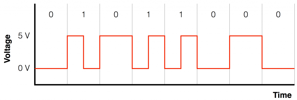
As we saw in the first posting, an S-PDIF signal uses a bi-phase mark, which is the same as saying it’s a frequency-modulated square wave where a “1” is represented by a square wave with double the frequency of a “0”. So, for example, Figure 1 shows one possible representation of the sequence 01011000. (The other possible representation would be the same as this, but upside down, because the first “0” started as a high voltage value.
If that square wave were sent through a wire that rolled off the high frequencies, then the result on the other side might look something like Figure 2.
If we use a detection algorithm that is looking for the moment in time when the incoming signal crosses what we expect to be the half-way point between the high and low voltages, then we get the following
As you can see in Figure 3, the time the transition is detected is late (which is okay) and it varies with respect of the correct time (which is not okay). That variation is the jitter that is caused by the relationship between the pattern in the bi-phase mark, the fundamental frequency of the “square wave” of the carrier (which is related to the sampling rate and the word length, possibly), and the cutoff frequency of the low-pass filter.
Duty Cycle Distortion
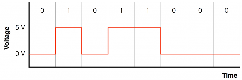
Typically, a digital signal is transmitted using some kind of pulse wave (which is the correct term for what I’ve been calling a “square wave”. It’s a square-ish wave (in that it bangs back and forth between two discrete voltages) but it’s not a square wave because the frequency is not constant. This is true if it’s a non-return-to-zero strategy (where a 1 is represented by a high voltage and a 0 is represented by a low voltage, as shown in Figure 4) or a bi-phase mark (as shown in Figure 1).
In either of these two cases (NRZ or bi-phase mark), the system modulates the amount of time the pulse wave is a high voltage or a low voltage. This modulation is called the duty cycle of the pulse wave. You’ll sometime see a “duty cycle” control on a square wave generator which lets you adjust whether the pulse wave is a square wave (a 50% duty cycle – meaning that it’s high 50% of the time and low 50% of the time) or something else (for example, a 10% duty cycle means that it’s high 10% of the time, and low 90% of the time)
If your transmission system is a little inaccurate, then it could have an error in controlling the duty cycle of the pulse wave. Basically, this means that it makes the transitions at the wrong times for some reason, thus creating a jittered signal before it’s even transmitted.
Echo Jitter
We’re all familiar with an echo. You stand far enough away from a wall, you clap your hands, and you can hear the reflection of the sound you made, bouncing back from the wall. If the wall is far enough away, then the echo is a second, separate sound from the original. If the wall is close, you still get an echo (in fact, it’s even louder) but it’s coming at you so soon after the original, direct sound, that you can’t perceive it as a separate thing.
What many people don’t know is that, if you stand in a long corridor or a tunnel with an open end, you will also hear an echo, bouncing off the open end of the tunnel. It’s not intuitive that this is true, since it looks like there’s nothing there to bounce off of, but it happens. A sound wave is reflected off of any change in the acoustic properties of the medium it’s travelling through. So, if you’re in a tunnel, it’s “hard” for the sound wave to move (because there aren’t many places to go) and when it gets to the end and meets a big, open space, it “sees” this as a change and bounces back into the tunnel.
Basically, the same thing happens to an electrical signal. It gets sent out of a device, runs down a wire (at nearly the speed of light) and “hits” the input of the receiver. If that input has a different electrical impedance than the output of the transmitter and the wire (on other words, if it’s suddenly harder or easier to push current through it – sort of….) then the electrical signal will (partly) be reflected and will “bounce” back down the wire towards the transmitter.
This will happen again when the signal bounces off the other end of the wire (connected to the transmitter) and that signal will head back down the wire, back towards the receiver again.
How much this happens is dependent on the impedance characteristics of the transmitter’s output, the receiver’s input, and the wire itself. We will not get into this. We will merely say that “it can happen”.
IF it happens, then the signal that is arriving at the receiver is added to the signal that has already reflected off the receiver and the transmitter. (Of course, that combined signal will then be reflected back towards the transmitter, but let’s pretend that doesn’t happen.)
The sum of those two signals is the signal that the receiver tries to decode into a carrier signal. However, the reflected “echo” is a kind of noise that infects the correct signal. This, in turn, can cause timing errors in the detection system of the receiver’s input.
Periodic Jitter
Let’s take a CD player’s S-PDIF output and connect it to the S-PDIF input of a DAC. We’ll use an old RCA cable that we had lying around that has been used in the past – not only as an audio interconnection, but also to tie a tomato plant to a trellis. It’s also been run over a couple of times, under the wheels of an office chair. So, what was once a shield made of nice, tightly braided strands of copper is now full of gaps for electromagnetic waves to bleed in.
We press play on the CD, and the audio signal, riding on the S-PDIF carrier wave is sent through our cable to the DAC. However, the signal that reaches the DAC is not only the S-PDIF carrier wave, it also contains a sine wave that is radiating from a nearby electrical cable that is powering the fridge…
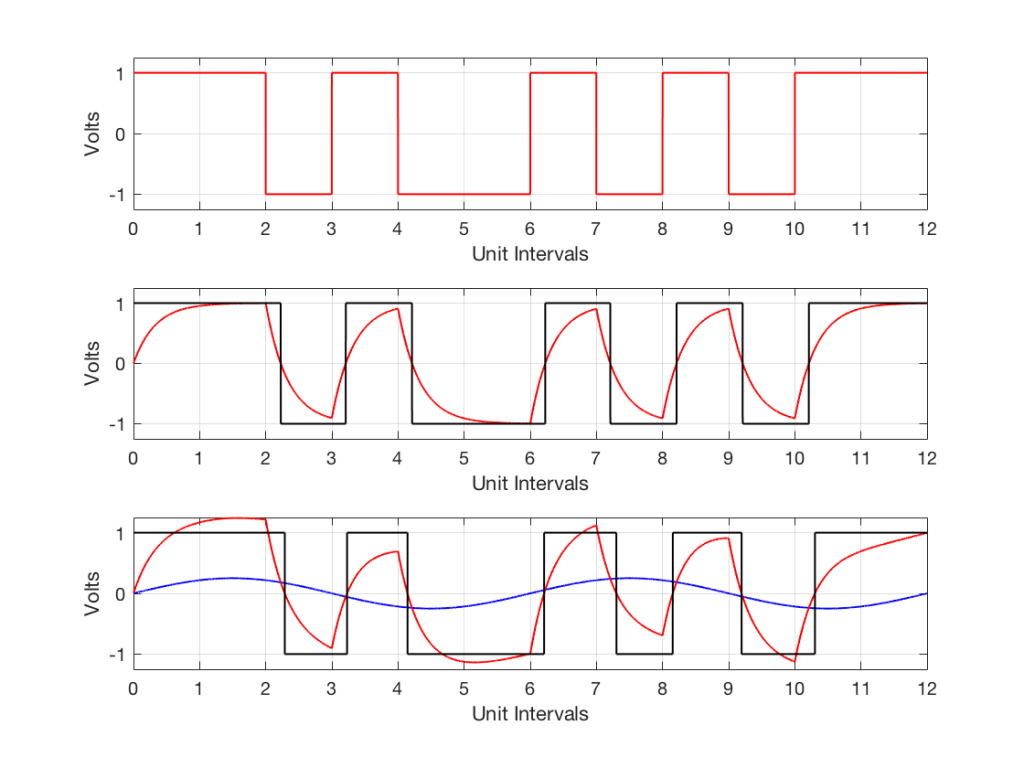
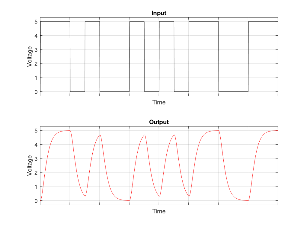
Take a look at Figure 5. The top plot, in red, is the “perfect” carrier wave, sent out by the transmitter.
If that wave is sent through a system that rolls off the high end, the result will look like the red curve in the middle plot. This will be trigger clock events in the receiver, shown as the black curve in the middle plot. There, you may be able to see the intersymbol interference jitter (although it’s small, and difficult to see in that plot).
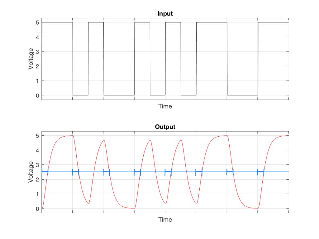
The blue curve in the bottom plot shows the sinusoidal modulator coming into the system from an external source. That’s added to our low-pass filtered signal, resulting in the red curve in the bottom plot (see how it appears to “ride” the blue curve up and down). The black curve is the end result, triggered by the instances when the red line crosses the mid-point (in this plot, 0 V). You should be able to see there that when the sinusoid is positive, the trigger event is late (relative to what it would have been – the black curve in the middle plot). When the sinusoid is negative, the trigger event is early.
Putting some of it together…
If we take a system that is suffering from
- Intersymbol Interference (Deterministic)
- Periodic Jitter (Deterministic)
- Random Jitter
Then the result looks something like Figure 6.
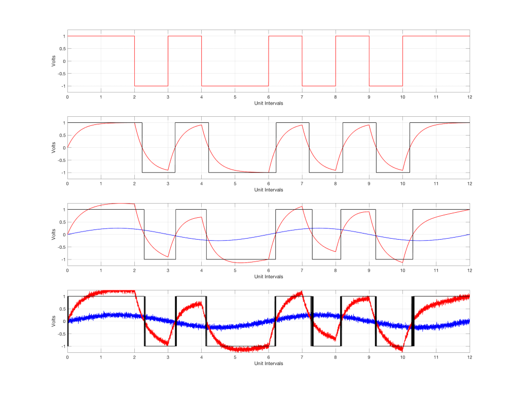
The top plot shows the original bi-phase mark that we intend to transmit.
The second plot shows the low-pass filtered carrier wave (in red) and the triggered events that result (in black).
The third plot shows the periodic, sinusoidal source (in blue), the resulting carrier wave (in red) and the triggered events that result (in black).
The bottom plot adds random noise to the sinusoid (in blue), therefore adding noise to the carrier wave (in red) and resulting in indecision on the transition time. This is because, when the noisy carrier wave crosses the threshold, it goes back and forth across it multiple times per “transition”. So, the black wave is actually banging back and forth between the “high” and “low” values a bunch of times, each time the carrier crosses the threshold. If you are going to build a digital audio receiver that is reasonably robust, you will need to figure out how to deal with this smarter than the way I’ve shown it here.
Addendum: S-PDIF data vs cable lengths
One of the factors to worry about when you’re thinking about Echo Jitter is the “wavelength” of one “cell”. A cell is the shortest duration of a pulse in the wave (which is half of the duration of a bit – the “high” or the “low” value when transmitting a value of 1 in the bi-phase mark).
This is similar to a real echo in real life. If you clap your hands and hear a distinct echo, then the reflecting surface is very far away. If the echo is not a separate sound – if it appears to occur simultaneously with the direct sound, then the wall is close.
Similarly, if your electrical cable is long enough, then a previous value (a high or a low voltage) may be opposite to the current value sometimes – which may have an effect on the signal at the input of the receiver.
This raises the question: how long is “long”? This can be calculated by finding the wavelength of one cell in the electrical cable when it’s being transmitted.
The speed of an electrical signal in a good conductor is approximately 299,792,458 m/s.
The number of cells per second in an S-PDIF transmission can be calculated as follows:
sampling rate * number of audio channels * 32 bits/frame * 2 cells/bit
This means that the number of cells per second are as follows:
| Fs | Cells per Second |
| 44.1 kHz | 5,644,800 |
| 48 kHz | 6,144,000 |
| 88.2 kHz | 11,289,600 |
| 96 kHz | 12,288,000 |
| 176.4 kHz | 22,579,200 |
| 192 kHz | 24,576,000 |
If we divide the speed of a wave on a wire by the number of cells per second, then we get the length of one cell on the wire, which turns out to be the following:
| Fs | Cell length |
| 44.1 kHz | 53.1 m |
| 48 kHz | 48.8 m |
| 88.2 kHz | 26.6 m |
| 96 kHz | 24.4 m |
| 176.4 kHz | 13.3 m |
| 192 kHz | 12.2 m |
So, even if you’re running S-PDIF at 192 kHz AND if you are getting an echo on the wire (which means that someone hasn’t done a very good job at implementing the correct impedances of the S-PDIF output and input): if your interconnect cable is 30 cm long then you don’t need to worry about this very much (because 30 cm is quite small relative to the 12.2 m cell length on the wire…)