#4 in a series of articles about wander and jitter
Dig out your old cassette copy of “Love Will Keep us Together”, performed by Captain and Tenille (although the original version was released by Neil Sedaka (one of the songwriters) in France) and press PLAY on your oldest cassette deck. You’ll hear the song (now it’s stuck in your head, isn’t it?) as well the hiss from the cassette. That hiss comes (mostly) from the random-ness of the magnetic tape itself, and is just a signal that is added to Captain and Tenille.
Random jitter is similar to the tape hiss. You have a signal (the audio signal that has been encoded as a digital stream of 1’s and 0’s, sent through a device or over a wire as a sequence of alternating voltages) and some random noise is added to it for some reason… (Maybe it’s thermal noise in the resistors, or cosmic radiation left over from the Big Bang bleeding through the shielding of your S-PDIF cable, or something else… )
That random noise results in the device (the audio gear or the chip inside it) wrongly interpreting what time it is, which may or may not affect your audio signal (we’ll talk about that later in the series).
The difference between the cassette example and jitter is that the noise that is modulating the “signal” is not really added to it (at least, it’s not added to the audio signal…). What we’re really talking about is that the jitter is modulating the signal that carries your audio signal – not the audio signal itself. This is an important distinction, so if that last sentence is a little fuzzy, read it again until it makes sense.
Good, I assume that if you’re gotten to this sentence, then you know the difference between the audio signal (the sound of Captain and Tenille singing “Love Will Keep us Together”) and the Carrier signal that is delivering the data that contains that audio signal.
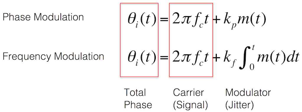
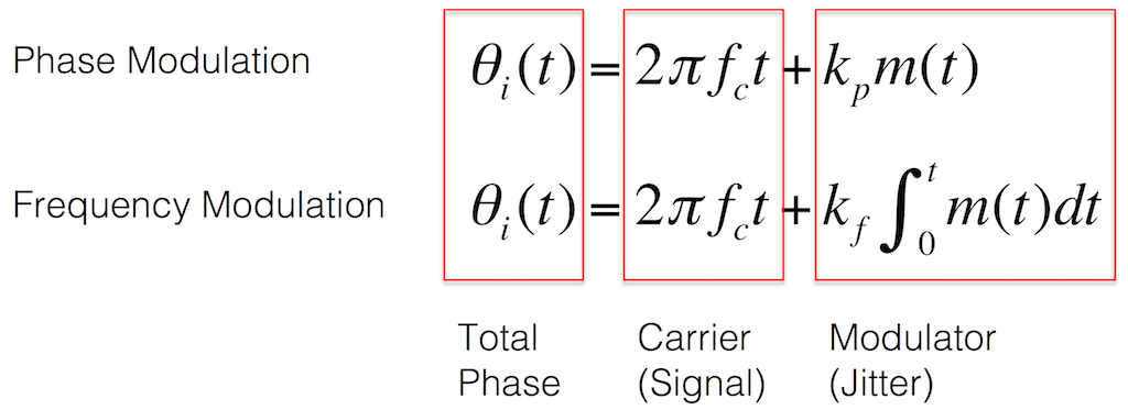
This means that we can talk about the Carrier (for example, the S-PDIF stream of bits that carries the digitally-encoded audio signal) and the Modulator (the signal that changes the timing of that carrier coming in, and thus resulting in jitter).
- Timing errors of the clock events relative to their ideal positions
- Timing errors of the clock periods relative to their ideal lengths in time
These are very different – although they look very similar.
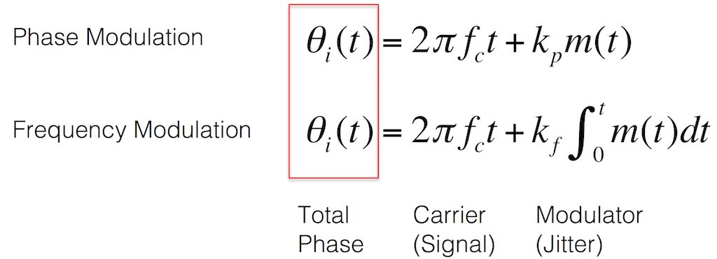
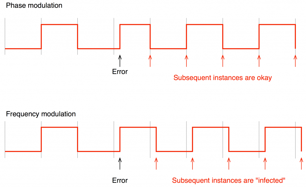
The first is an absolute measure of the error in the clock event – when did that single event happen relative to when it should have happened? Each event can be measured individually relative to perfection – whatever that is. This is called a Phase Modulation of the carrier. It has a Gaussian characteristic (which I’ll explain below…) and has no “memory” (which is explained first).
The second of these isn’t a measure of the events relative to perfection – it’s a measure of the amount of time that happened between consecutive events. This is called a Frequency Modulation of the carrier. It also has a Gaussian characteristic (which I’ll explain below…) but it does have a “memory” (which is explained using Figure 1).
Gaussian Distribution
If you stood on a street in New York City and asked the first 100,000 people you saw how much they spent on buying their last car, you would get a very wide range of answers. A very few people who say that they spent a LOT of money. A very few people would say that they spent nothing because they don’t own a car. Most people would give you around the same number, give or take. If we took all of those answers, grouped them into ranges of $100, and plotted the results (therefore showing how many people bought a car that cost $0 – $100, $101 – $200, $201 – $300, and so on… you’d get something like the graph shown in Figure 2.
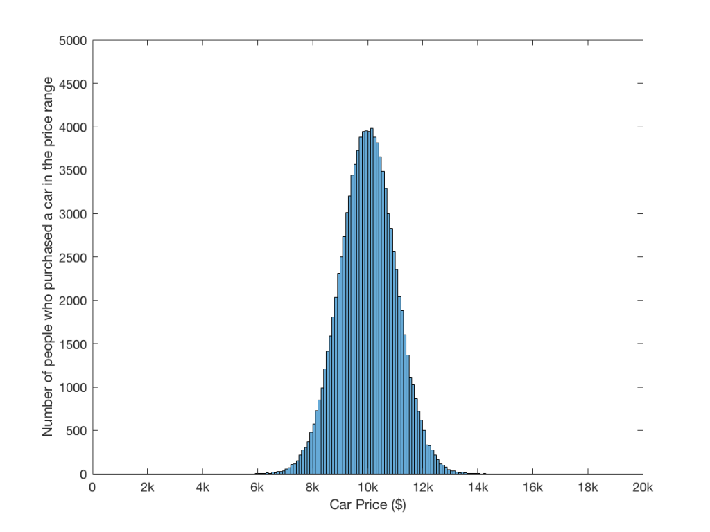
As you can see in the plot in Figure 2, most people spent about $10,000 on their last car. Some some spent more, some spent less… But the further you get from $10,000, the fewer people are “in the club”.
Of course, I made up those numbers – but the important thing is not the actual data – it’s the shape it makes. That “bell curve” is called a “normal distribution” or a “Gaussian distribution” of numbers. If you graph things that occur in nature – everyone’s age in the whole world, the brightness of stars, math grades in Canadian grade 6 students’ final exams, heights of all plants – you’ll see this shape often.
Okay, I lied a little… If you take the ages of everyone in the world, or the heights of all plants, you won’t really get a true Gaussian distribution. This is because, if the values (the ages or the heights) really had a Gaussian distribution, then it would be possible for them to be infinite. Admittedly, the probability of the value being infinite is infinitely small – but that’s a small detail… In addition, the distribution would have to be symmetrical, and since it should be possible to have a value ∞, that would mean that it should also be possible to have a value of -∞ as well…
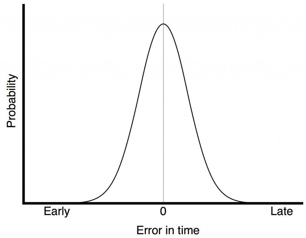
Let’s get back to Random Jitter… If the jitter is truly random, and we measure the errors in the time events, we will see a Gaussian distribution, centred at 0 seconds. In other words, the error has the highest probability of being 0 (and therefore no error) and the bigger the error (either too early or too late) the smaller the probability of that happening. Weirdly, since the distribution is Gaussian (or at least, we assume that it is) then the worst-case error is -∞ or ∞ – in other words, the event might never happen for some reason – no matter how long you wait…
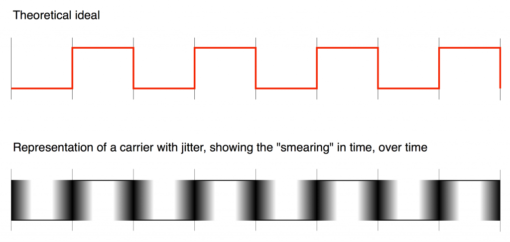
This means that, if you plot a jittered carrier wave on a display, and take a long-exposure photograph of it, you’ll see how the timing events move in time as a “blur” in the photo. A simple artist’s conception (yes, I phrased that correctly…) of this is shown in Figure 4.
Addendum: A little bit of math…
This is just a little extra information for geeks and aspiring geeks. If this gives you a headache, ignore it. It will not help you.

