#95 in a series of articles about the technology behind Bang & Olufsen
Imitation is the highest form of flattery
We attended a concert last week at the Danish Guitar Camp, where Carlo Marchione played a collection of music written for various instruments in the 1700s. One of those pieces was an arrangement of the Adagio from Mozart’s Klaviersonate in B-Major K. 570, which I had never heard before.
As soon as he started, I thought…. waitaminute…. this tune sounds awfully familiar… as a Canadian…
wait… what?
Have a listen to the first 10 seconds of the Mozart, then listen to the first 10 seconds of the Canadian National Anthem. I suspect that Calixa Lavallée might have had the Mozart tune in the back of his head when he sat down to work on Théodore Robitaille’s commission.
Making a violin
Making a cello
It’s not acoustics, but it’s close
Development of Beolab 90
#94 in a series of articles about the technology behind Bang & Olufsen
This was an online lecture that I did for the UK section of the Audio Engineering Society.
Perfect symmetry
When working on the last series of posts, I stumbled on a signal that caused an FFT analysis to look a little strange to me. This post is about that strangeness.
If I make a sine wave (in a floating point world) that sits perfectly on an FFT bin, and I do an FFT of it, the noise floor that I see is the result a lack of precision of the calculations that were used to make the signal. An example of this is shown in Figure 1.
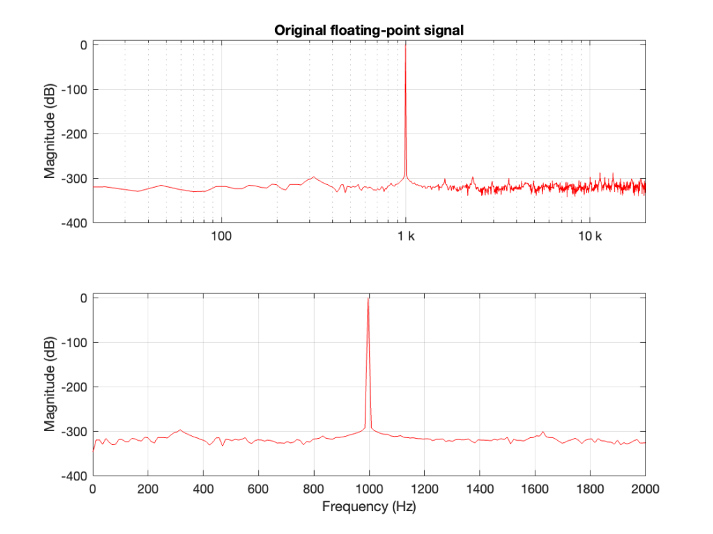
As can be seen there, the noise floor in the fit is typically at least 300 dB down from the signal level. This means that if the signal has a peak amplitude of 1, then each bin in my FFT has a peak amplitude of less than 0.000 000 000 000 001, which is very, very, low.
If I dither and quantise the sine wave with, say, a 24-bit LPCM precision, then the result would be different, as shown in Figure 2.
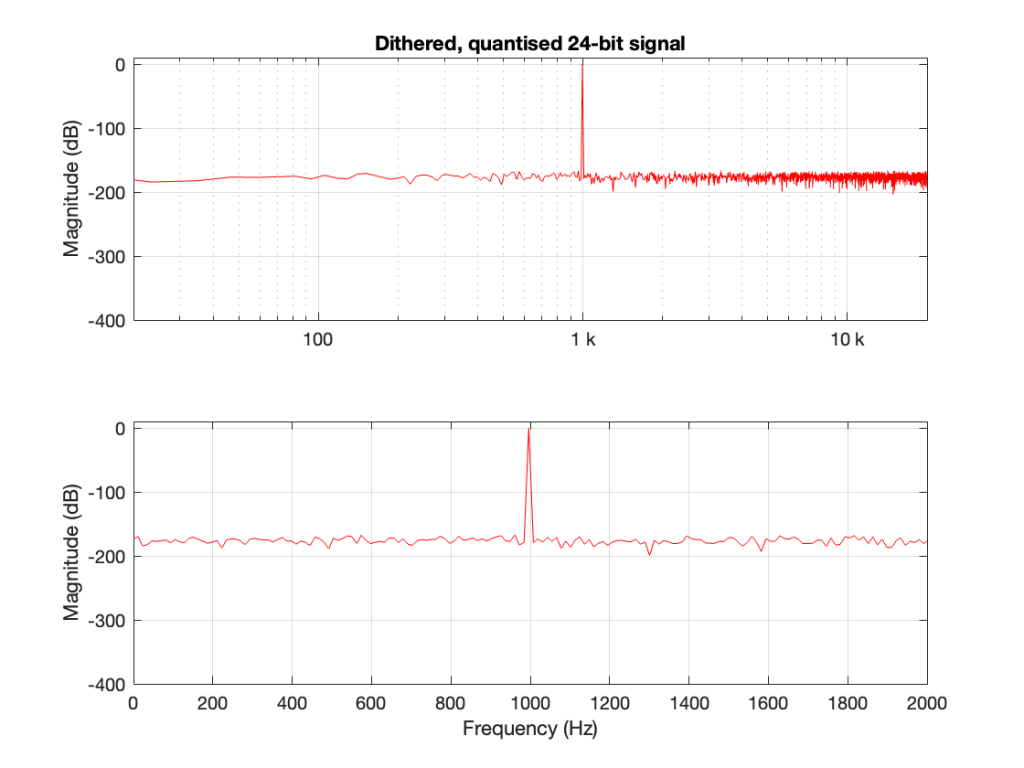
Now the noise floor seen in the FFT analysis is the noise that is intentionally generated as dither to randomise the quantisation error when converting to LPCM.
However, what happens if the signal is quantised but not dithered? Then the result looks like Figure 3.
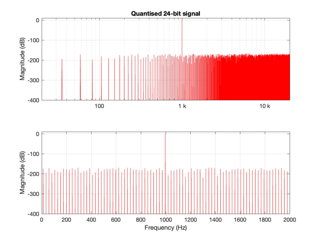
This is interesting because, starting the first bin, every second bin has nothing in it, so on a decibel scale, the value is -∞ dB. Why does this happen?
The short answer is symmetry. By quantising the sine wave, I made it perfectly symmetrical.
This removes the DC content, since the positive-going portion of the waveform is identical to the negative-going portion. Therefore there’s nothing at 0 Hz (which is DC) or any of its “harmonics” (at least in the world of FFT bins…).
There is content of some kind in the other bins because our sine wave is not perfectly sinusoidal. All those steps that I put in it are an error that generates information at frequency centres other than the sine tone’s itself.
So, if you do an FFT on a sinusoidal signal and you see a result where half of the bins have nothing in them, one possible reason is that you’re dealing with a perfectly symmetrical signal.
Excruciating minutiae: Part 4
I mentioned in this posting that lately I’ve been doing some measurements of a DUT that:
- required a frequency analysis with a very big dynamic range
- … which meant that I was testing it using a sine tone with a frequency that was exactly the same as an FFT bin’s frequency centre
- … and the sine tone had to be sent through the device by playing a standard audio file (wav and/or FLAC)
So, I did this, but I saw some weirdness that I didn’t expect down in the noise floor of the FFT output. Whenever I’m testing something and I see something weird, I start working my way back through the audio chain to verify that the weirdness is coming from the thing that I’m testing, and not from my test system itself.
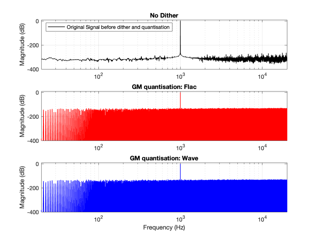
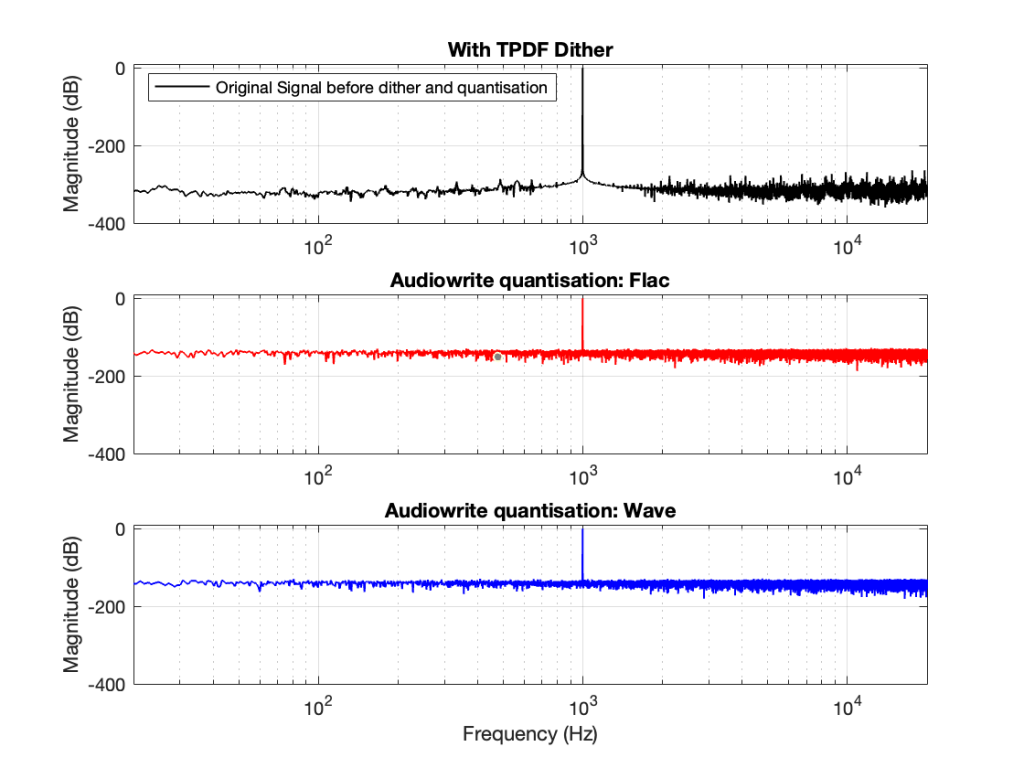
So, the first step was to do of an FFT of both the .wav and the .flac files that I was sending through the DUT. The results of this test looked something like Figure 1.
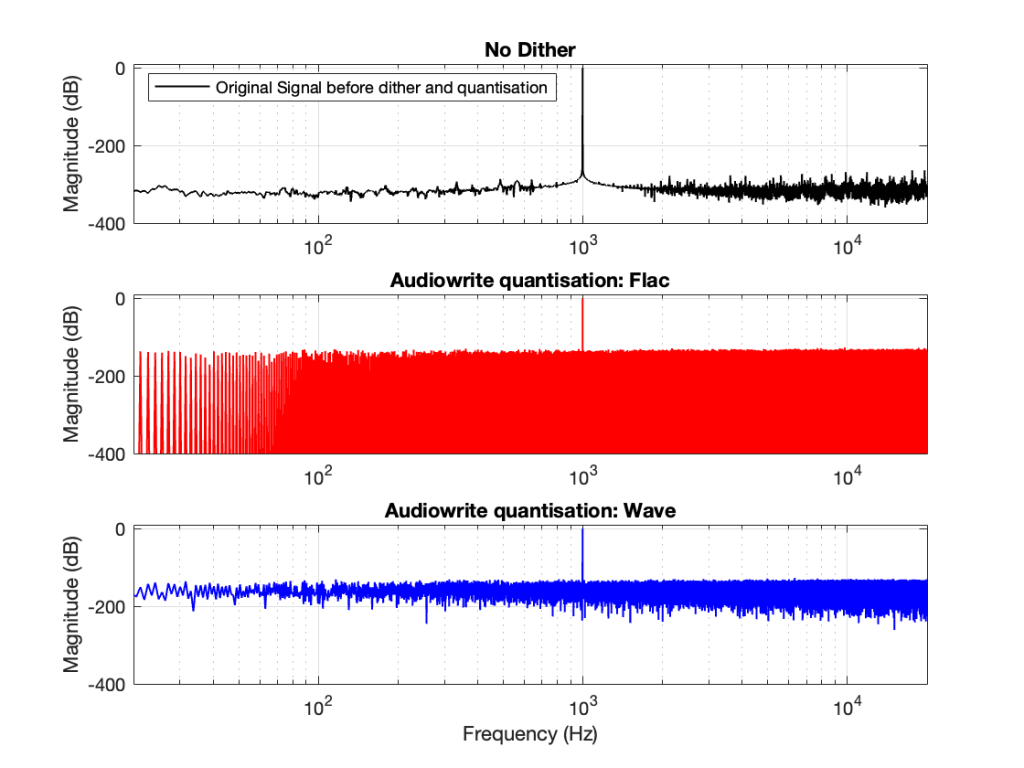
Before I go further, let’s clarify exactly what I did to generate those three plots.
- Using Matlab, I made a sine wave with a frequency identical to an FFT bin that was a close as possible to 997 Hz as I could get with a 65,536-point FFT at 48 kHz. (See this posting for more information about this.)
- I exported the signal using Matlab’s “audiowrite” function, both as a 24-bit wav and a 24-bit FLAC.
- I imported the two files back into Matlab
- I ran an FFT on the original, and the two imported files
I would not expect the bottom two plots to be as “good” as the top plot, since they’ve been reduced to a 24-bit fixed point version of the original floating-point signal. However, there are two things to notice in Figure 1.
- The most important thing is that the FLAC and WAVE imports produce different results. This is weird.
- The less-important (but more interesting, later…) thing is that, for the FLAC import, every odd-numbered FFT bin is -∞ dB, which means that there is absolutely NO energy at those frequencies.
First things first
Let’s address that first issue first. The FFTs show us that the signals coming back from the .wav and .flac import are different. But I’m interested in (1) how they’re different and (2) why they’re different.
Let’s try to answer the first question first. I made a linear ramp that had the same number of samples as the number of quantisation values and had a range of -1 to 1 (just like my sine wave…). So, to test a 16-bit export, I made a ramp that was 216 = 65,536 samples long (shown in the top plot in Figure 2). To test a 24-bit export, the ramp was 224 samples long.
In theory, if I export this ramp to a file type with the matching number of bits, then each sample should quantise to the next quantisation level from the bottom to the top. I then exported this ramp out to .wav and .flac, imported it again, and looked at the result, which is shown in Figure 2.
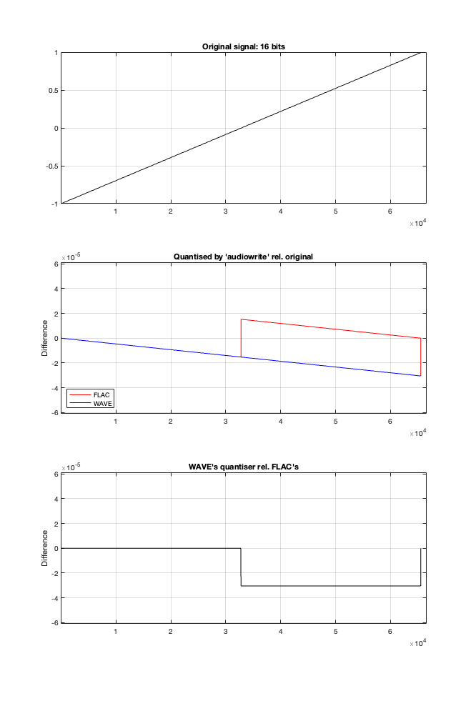
If I subtract the results of the imported files from the original, I get the result shown in the middle plot in Figure 2. I would NOT expect either the .wav or the .flac to be identical to the original, since information is lost in the export to a 16- or 24-bit fixed point LPCM format. However, I WOULD expect the .wav and .flac to be the same, which they obviously aren’t.
As can be seen in the bottom plot in Figure 2, there is a 1-quantisation level difference between the .wav and .flac files for signal values higher than 0.
Now the question is whether this difference is inherent in the file format, or if something else is going on. To test this, I did the same test on the 997-ish Hz sine wave (again) without dither, but with my own quantisation (using the code shown in this post). The result of this test is shown in Figure 3.
As you can see there, the imported .wav and .flac files behave identically. But, if you look carefully and compare to the .flac version in Figure 1, you’ll see that they’re different from THAT version.
The fact that the red and blue plots in Figure 3 are identical tell me that .wav and .flac are identical.
The fact that my quantisation results in identical results in .wav and .flac, but are different from Matlab’s “audiowrite” results (which produces .wav and .flac files that are different from each other) tells me that Matlab’s quantisation is different for .wav and .flac – and different from what I’m doing.
So, I go back to the ramp shown in Figure 2 and dig into the details again, zooming in on the samples near a value of -1, 0, and 1. These are shown below in Figure 4.
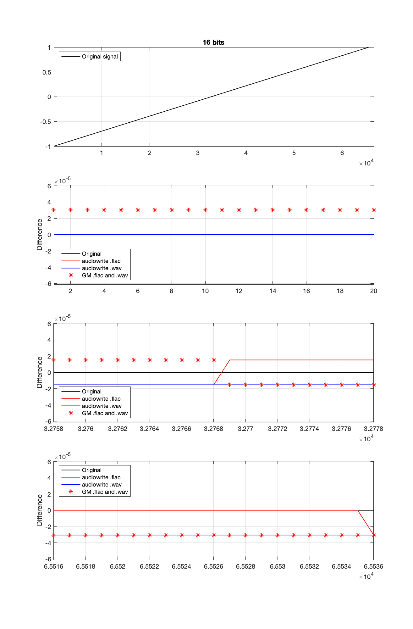
It’s a bit cryptic to see the results in Figure 4, but let’s walk through it.
- The top plot shows the ramp signal that I encoded as a 16-bit audio file in 4 different ways: as a .wav and a .flac, using audiowrite’s quantiser and mine.
- The second plot shows the differences in the imported files relative to the original for the first 20 samples, which correspond to the bottom 20 quantisation levels. As can be seen there, the audiowrite quantiser’s result appears to be identical to the original (they’re not, as we saw in the middle plot of Figure 1, but they’re close…). My quantiser is one level higher. This is because I’m scaling my original signal so that it can’t reach the bottom, as I talked about in Part 2.
- The third plot shows the behaviour of the three quantisers (2 audiowrites and mine) around the 0 value ±10 quantisation levels. Note that there’s no sample with a value of 0 (Because two’s complement is not symmetrical around the 0 value.). It’s not immediately obvious there, but all three quantisers have an “error” of 1/2 a quantisation level step around 0.
- Below 0, both of audiowrite’s quantisers have a negative offset, and mine has a positive offset.
- Above 0, audiowrite’s .flac quantiser has a positive offset whereas both audiowrite’s .wav quantiser and mine have a negative offset
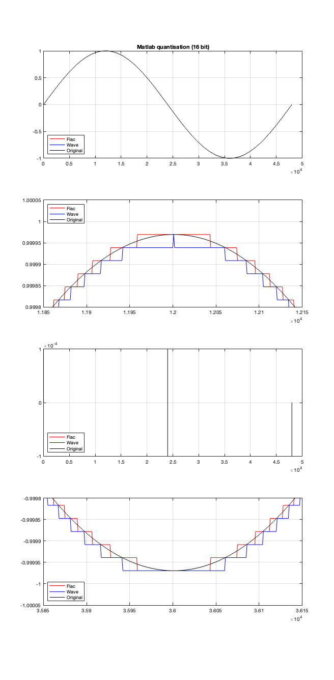
If the signal were a sine wave, then we’d see the same thing, it would just be harder to interpret, as shown in Figure 5. (There’s nothing useful shown in the third plot there because when you zoom in so closely , the slope of the sine wave as it passes 0 is really steep…)
I titled this series of posts “Excruciating minutiae” for a reason. The “error” (let’s call it a “difference” instead) is VERY small. It’s a difference of 1 quantisation level on a portion of the signal, which raises the very pragmatic question: “So what?”
Unless you’re REALLY digging into the bottom of the noise floor of a device, you probably never need to care about this. (In fact, even if you ARE digging into the bottom of the noise floor, you might not need to care.)
You CERTAINLY don’t have to worry about it if you’re just writing audio files to listen to, since you should be dithering those with TPDF dither, which will create a noise floor that is FAR above the “errors” caused by the differences I described above. This can be seen in Figures 6 and 7 below.

In other words, I’ve been using Matlab to export test files both in .wav and .flac for at least 20 years, and it’s only now that I’ve noticed this issue, which is another way of saying “don’t worry about it…”
Nota Bene
If you’re still awake, you might notice that there is one loose end… At the top of this posting I said
The less-important (but more interesting, later…) thing is that, for the FLAC import, every odd-numbered FFT bin is -∞ dB, which means that there is absolutely NO energy at those frequencies.
That will be the topic of another posting, since it’s more or less unrelated to this one – it was just an artefact of the test I described above.
Excruciating minutiae: Part 3
In Part 2 of this series, I wrote the following sentence:
The easiest (and possibly best) way to do this is to create white noise with a triangular probability distribution function and a peak-to-peak amplitude of ± 1 quantisation level.
That’s a very busy sentence, so let’s unpack it a little.
Rolling the dice
If you roll one die, you have an equal probability of rolling any number between 1 and 6 (inclusive). Let’s roll one die 100 times counting the number of times we get a 1, or a 2, or a 3, and so on up to 6.
| Number rolled | Number of times the number was rolled | Percentage of times the number was rolled |
| 1 | 17 | 17 |
| 2 | 14 | 14 |
| 3 | 15 | 15 |
| 4 | 15 | 15 |
| 5 | 21 | 21 |
| 6 | 18 | 18 |
(Note that the percentage of times each number was rolled is the same as the number of times each number was rolled only because I rolled the die 100 times.)
If I plot those results, it looks like Figure 1.
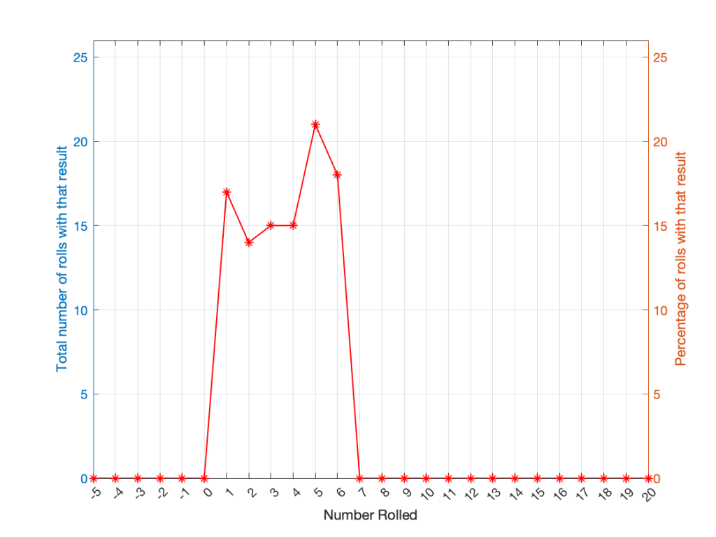
It may be weird, but I’ve plotted the number of times I rolled -5 or 13 (for example). These are 0 times because it’s impossible to get those numbers by rolling one die. But the reason I put those results in there will make more sense later.
Let’s keep rolling the die. If I do it 1,000,000 times instead of 100, I get these results:
| ed | Number of times the number was rolled | Percentage of times the number was rolled |
| 1 | 166225 | 16.6225 |
| 2 | 166400 | 16.6400 |
| 3 | 166930 | 16.6930 |
| 4 | 167055 | 16.7055 |
| 5 | 166501 | 16.6501 |
| 6 | 166889 | 16.6889 |
Now, since I rolled many, many, more times, it’s more obvious that the six results have an equal probability. The more I roll the die, the more those numbers get closer and closer to each other.
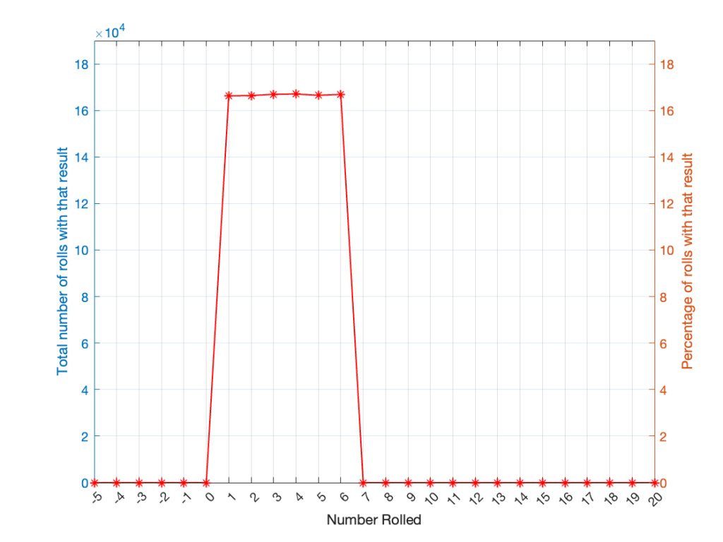
Take a look at the shape of the plot above. The area under the line from 1 to 6 (inclusive) is almost a rectangle because the six numbers are all almost the same.
The shape of that plot shows us the probability of rolling the six numbers on the die, so we call it a probability density function or PDF. In this case, we see a rectangular PDF.
But what happens if we roll two dice instead? Now things get a little more complicated, since there is more than one way to get a total result, as shown in the table below.
| Total | ||||||
| 2 | 1+1 | |||||
| 3 | 1+2 | 2+1 | ||||
| 4 | 1+3 | 2+2 | 3+1 | |||
| 5 | 1+4 | 2+3 | 3+2 | 4+1 | ||
| 6 | 1+5 | 2+4 | 3+3 | 4+2 | 5+1 | |
| 7 | 1+6 | 2+5 | 3+4 | 4+3 | 5+2 | 6+1 |
| 8 | 2+6 | 3+5 | 4+4 | 5+3 | 6+2 | |
| 9 | 3+6 | 4+5 | 5+4 | 6+3 | ||
| 10 | 4+6 | 5+5 | 6+4 | |||
| 11 | 5+6 | 6+5 | ||||
| 12 | 6+6 |
As can be (hopefully) seen in the table, there is only one way to roll a 2, and there’s only one way to roll a 12. But there are 6 different ways to roll a 7. Therefore, if you’re rolling two dice, it’s 6 times more likely that you’ll roll a 7 than a 12, for example.
If I were to roll two dice 1,000,000 times, I would get a PDF like the one shown in Figure 3.
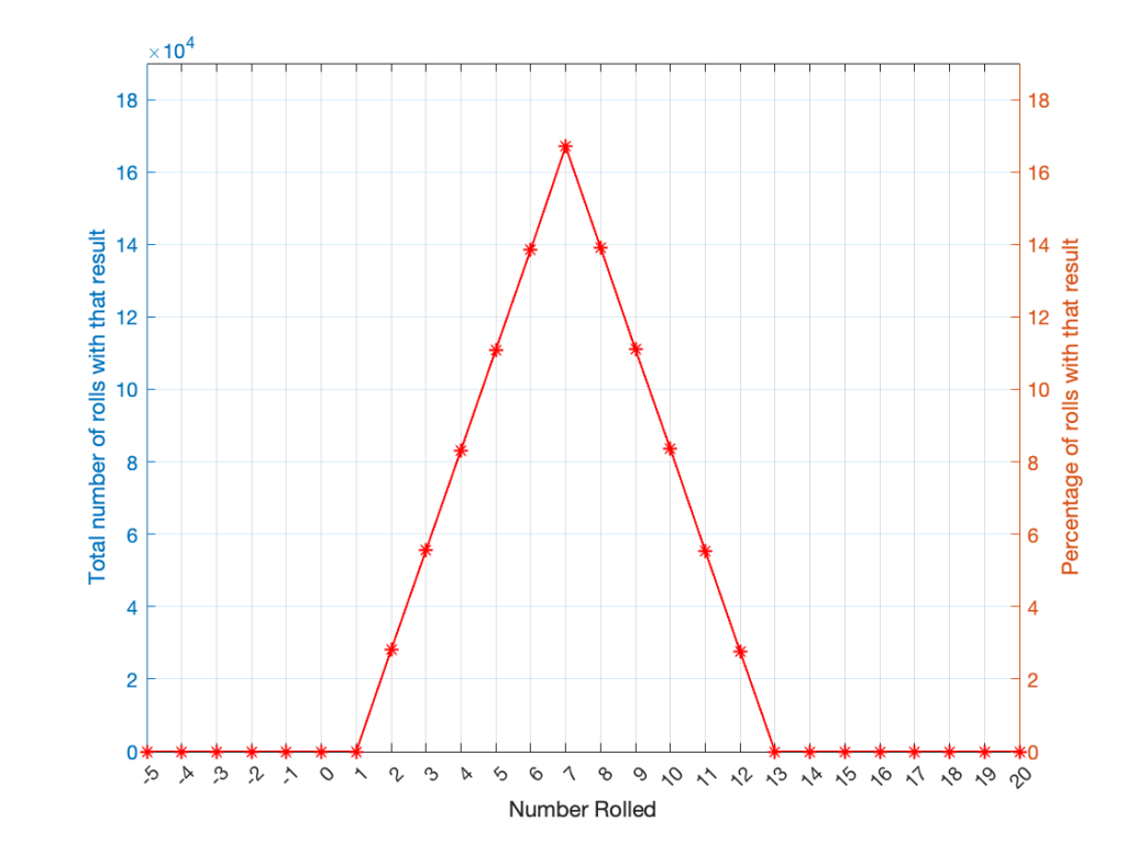
I won’t explain why this would be considered to be a triangular PDF.
Whether you roll one die or two dice, the number you get is random. In other words, you can’t use the past results to predict what the next number will be. However, if you are rolling one die, and you bet that you’ll roll a 6 every time, you’ll be right about 16.7% of the time. If you’re rolling two dice and you bet that you’ll roll a 12 every time, you’ll only be right about 2.8% of the time.
Let’s take two dice of different colours, say, one red die and one blue die. We’ll roll both dice again, but instead of adding the two values, we’ll subtract the blue value from the red one. If we do this 1,000,000 times, we’ll get something like the results shown below in Figure 4.
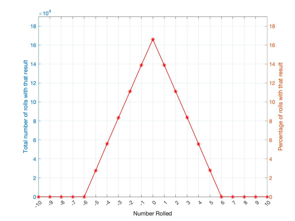
Notice that the probability density function keeps the same shape, it’s just moved down to a range of ±5 instead of 2 to 12.
Generating noise
In audio, noise is a sound that is completely random. In other words, just like the example with the dice, in a digital audio signal, you can’t predict what the next sample value will be based on the past sample values. However, there are many different ways of generating that random number and manipulating its characteristics.
Let’s start with a computer algorithm that can generate a random number between 0 and 1 (inclusive) with a rectangular PDF. We’ll then ask the algorithm to spit out 1,000,000 values. If the numbers really are random, and the computer has infinite precision, then we’ll probably get 1,000,000 different numbers. However, we’re not really interested in the numbers themselves – we’re interested in how they’re distributed between 0.00 and 1.00. Let’s say we divide up that range into 100 steps (or “buckets”) that are 0.01 wide and count how many of our random numbers fall into each group. So, we’ll count how many are between 0.0 and 0.01, between 0.01 and 0.02, and so on up to 0.99 to 1.00. We’ll get something like Figure 5.
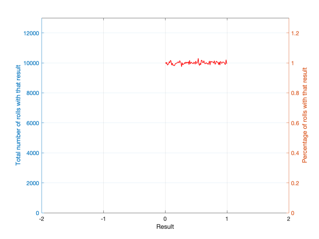
I’ve only plotted the probabilities of the possible values: 0 to 1, which winds up showing only the top of the rectangle in the rectangular PDF.
If I generate 1,000,000 random numbers with that algorithm, and then subtract 1,000,000 other random numbers, one by one, and find the probabilities of the result, the answer will be familiar.
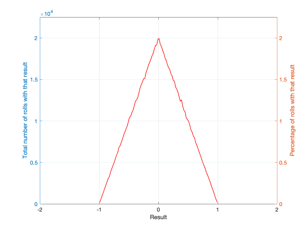
So, this is how we make the noise that’s added to the signal. If, for each sample, you generate two random numbers (making sure that your algorithm has a rectangular PDF) and subtract one from the other, you have the dither signal that will have a maximum level of ±1 quantisation level.
- The signal (with a maximum range of ±1) is scaled up by multiplying it by 2(NumberOfBits-1)-2
- then you add the result of the dither generator
- then the total is rounded to the nearest integer value
- and then the result is scaled back down by a factor of 2(NumberOfBits-1) to bring its back down to a range of ±1 to get it ready for exporting to a standard audio file format like .wav or .flac.
In other words, assuming that you have an audio signal called “Signal” that has a range of ±1 and consists of floating point values:
ScaleUp = 2^(Bitdepth-1)-2
ScaleDown = 2^(Bitdepth-1)

TpdfDither = rand(LengthOfSignal) - rand(LengthOfSignal)

QuantisedDitheredSignal = round(Signal * ScaleUp + TpdfDither) / ScaleDown;Excruciating minutiae: Part 2
In Part 1, I talked about how an audio signal is quantised, and how the world that the quantised signal lives in is slightly asymmetrical.
Let’s stay in a 3-bit world (to keep things comprehensible on a human scale) and do some recreational quantisation. We’ll start by making a sine wave with a peak amplitude of 1. This means that the total range will be ±1.
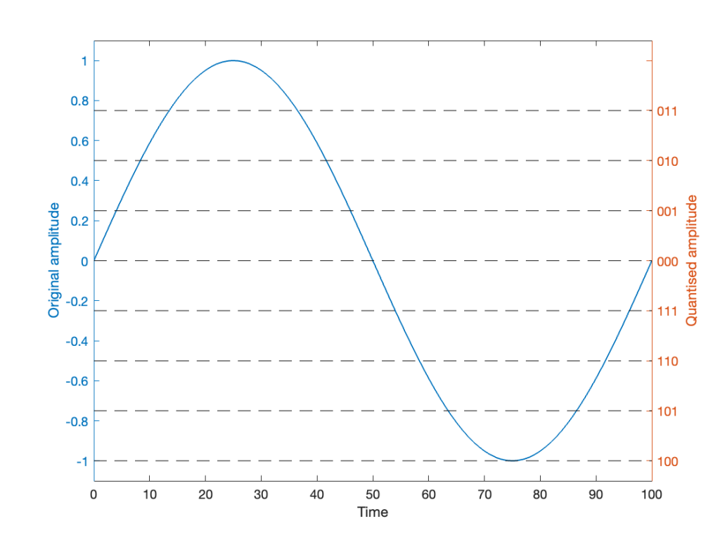
Notice that I put two scales on the plot in Figure 1. On the left, we have the “floating point” amplitude scale. On the right, we have the 8 quantisation levels.
If we are a bit dumb, and we just quantise that sine wave directly, making sure that I’ve aligned the scaling to use ALL possible quantisation values, we get the result in Figure 2.
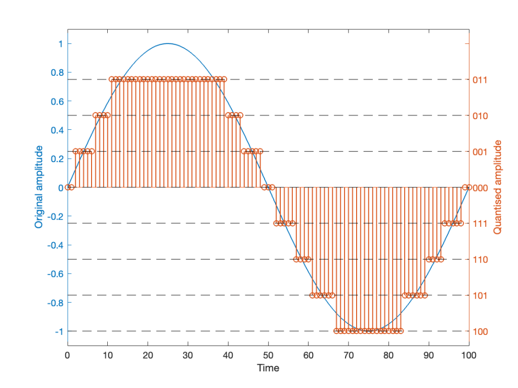
Notice that, because the original signal is symmetrical (with respect to positive and negative amplitudes) but the quantisation steps are not, we wind up getting a different result for the positive values than the negative values. In other words, after quantisation, I’ve clipped the positive peaks of the original signal.
Okay, so this is a dumb way to do this. A slightly less dumb way is to adjust the scaling so that the original wave does not use all possible quantisation values, as shown in Figure 3.
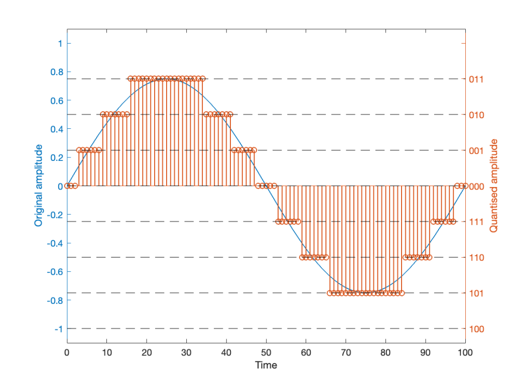
Notice that I’ve set the sine wave to a slightly lower level, so that it rounds to the top-most positive quantisation level, but this means that it doesn’t use the lowest negative quantisation level. If we’re being really picky, I could have made the sine wave just a little higher in amplitude: by 1/2 of a quantisation step, and the quantised result would still not have clipped asymmetrically.
Dither
As you can see in Figures 2 and 3 above, just taking a signal and quantising it generates an error. The more bits you have in the word length, the more quantisation levels you have, and the smaller the error. However, that error will always be correlated with the signal somehow, and as a result, it’s distortion, which is easy to learn to hear.
If, however, we add a little noise to the signal before we quantise it, then we can randomise the error, which changes the error from producing distortion to a constant signal-independent noise floor. Since the noise makes the quantiser appear to be indecisive, we call it dither.
The easiest (and possibly best) way to do this is to create white noise with a triangular probability distribution function and a peak-to-peak amplitude of ± 1 quantisation level. I’ll explain what that last sentence means in Part 3 of this series.
If we do this, then we
- take the signal
- add a little noise to it
- quantise it
and the result might look like Figure 4.
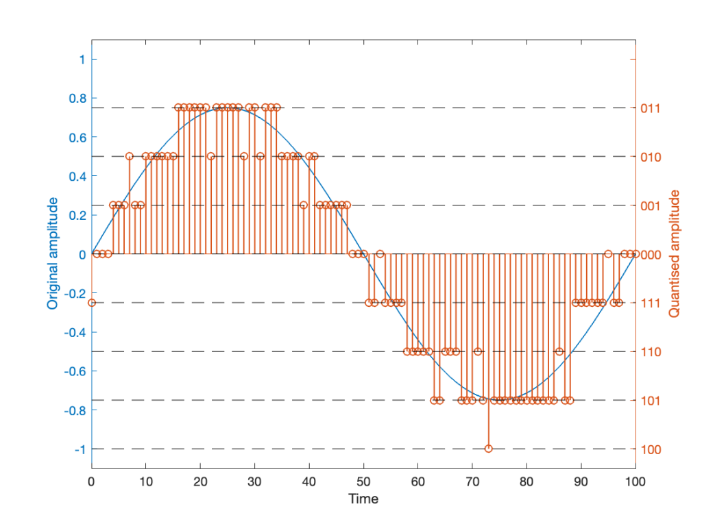
It should be easy to see that we still have quantisation, and also that I’ve added some random element to the signal.
However, let’s look at the mistake I made in Figure 4. The noise that was added to the signal has an amplitude of ±1 quantisation level. So, we should see cases where the signal looks like it should be rounding to the closest level, but it might be either 1 above or 1 below. (For example, take a look at Time = 70, 71, and 72 as an example of this.)
However, take a look around Time = 20 to 30. Notice that the original signal is close to the top quantisation level. This means that, although a negative value in the dither in those samples can bring the quantisation level down, a positive value cannot bring it up because we don’t have any room for it. This will, again, result in a small amount of asymmetrical clipping. This is a VERY small amount. (Remember that, in the real world we’re probably using 216 (= 65,536) or 224 (= 16,777,216) quantisation values, not 23 (= 8).
So, if we’re going to avoid this clipping, we need to adjust the scaling of the signal once more, as shown in Figure 5.
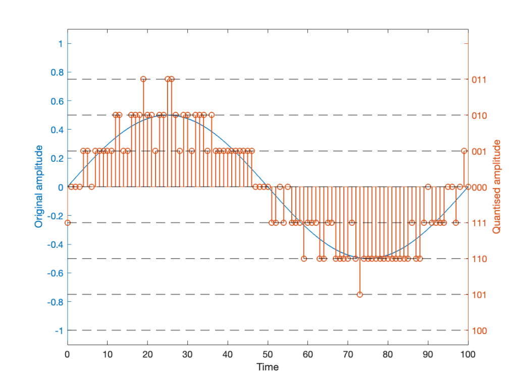
This shows a signal that is scaled so that, without dither, it would round to one level away from the top-most quantisation level. When you add the dither, it can go up to that top quantisation level. (In fact, I happened to use the same dither signal for Figures 4 and 5. The only difference is the scaling of the signal.)
Now, I know that if you’re not used to looking at 3-bit signals, and/or if dither is a new concept, the red signal in Figure 5 might make you a little upset. However (and you have to believe me on this…) this is the correct way to encode digital audio. Just because it looks crazy doesn’t mean that it is.
NB: The math
If you want to make the plots above, here’s a simplified version of the math to try it out. Note: I live in a world where a % symbol precedes a comment.
Some Constants
Bitdepth = 3
Fs = 100 % sampling rate in Hz
Fc = 1 % frequency of the sine wave in Hz
TimeInSamples = [0:Fs] % This will make the TimeInSamples all of the integer values from 0 to Fs (therefore, 1 second of audio)
Figure 1
Signal = sin(2 * pi * Fc/Fs * TimeInSamples)Figure 2
ScaleUp = 2^(Bitdepth-1)
ScaleDown = 2^(Bitdepth-1)

QuantisedSignal = round(Signal * ScaleUp) / ScaleDown;

% Then apply a clipper to remove the top quantisation level.
% You can do this yourself.
Figure 3
ScaleUp = 2^(Bitdepth-1)-1
ScaleDown = 2^(Bitdepth-1)

QuantisedSignal = round(Signal * ScaleUp) / ScaleDown;
Figure 4
ScaleUp = 2^(Bitdepth-1)-1
ScaleDown = 2^(Bitdepth-1)
TpdfDither = rand(LengthOfSignal) - rand(LengthOfSignal)

QuantisedDitheredSignal = round(Signal * ScaleUp + TpdfDither) / ScaleDown;

% Then apply a clipper to remove the top quantisation level.
Figure 5
ScaleUp = 2^(Bitdepth-1)-2
ScaleDown = 2^(Bitdepth-1)
TpdfDither = rand(LengthOfSignal) - rand(LengthOfSignal)

QuantisedDitheredSignal = round(Signal * ScaleUp + TpdfDither) / ScaleDown;