Now we’ve seen that if we have a filter that results in either a peak or a dip in the magnitude response, we’ll also result in the signal ringing in time. We’ve also seen that the frequency of the ringing is the centre frequency of the filter. Now let’s dig a little deeper into the behaviour of that ringing; or, more specifically its decay characteristics.
We’ll repeat the process from Part 2: measure the impulse response of a peaking filter where Fc = 1 kHz, gain = +12 dB, and Q = 2. However, this time I’ll look at the time response with a different scaling. Instead of plotting the linear value over time, I’ll convert each instantaneous value to dB and plot that. This looks like Figure 1.
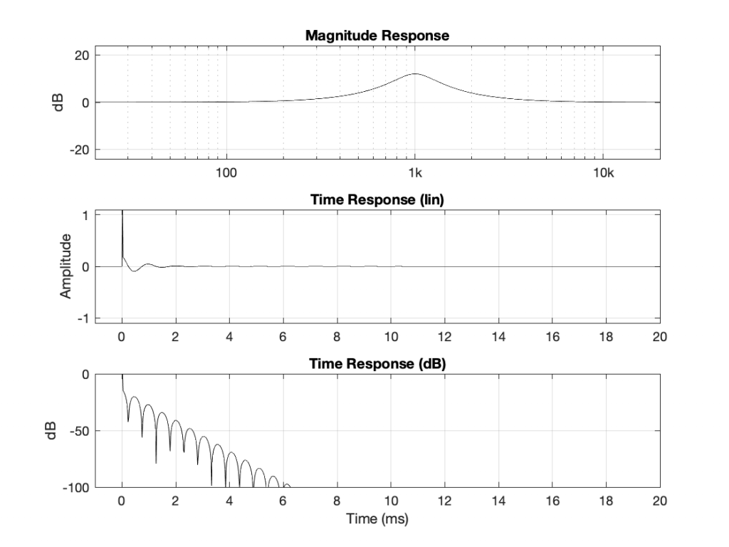
The important thing to notice here is that, when I plot the instantaneous amplitude in decibels (in other words, on a logarithmic scale), the decay is a straight line with a slope.
Let’s get two things out of the way here. This isn’t really decibels, because decibels requires some time averaging. Also, I’m actually plotting the absolute value of the impulse response in a decibel scale, because if I try to calculate the log of a negative number, things get ugly. This means that the math I’m actually using to create the bottom plot is
20 * log10(abs(signal))
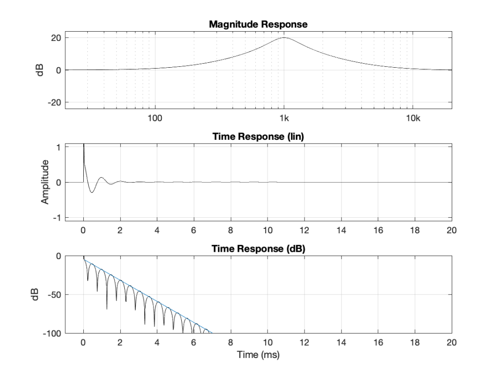
If I draw a line across the tops of the bumps in that plot, I can look at the decay of the filter’s ringing as in Figure 2.

For this filter, the decay rate of the ringing is -1360 dB per second (which is very fast). Let’s change some parameters and see what happens.
If I increase the gain of the filter without changing the Fc or the Q, I get the following:
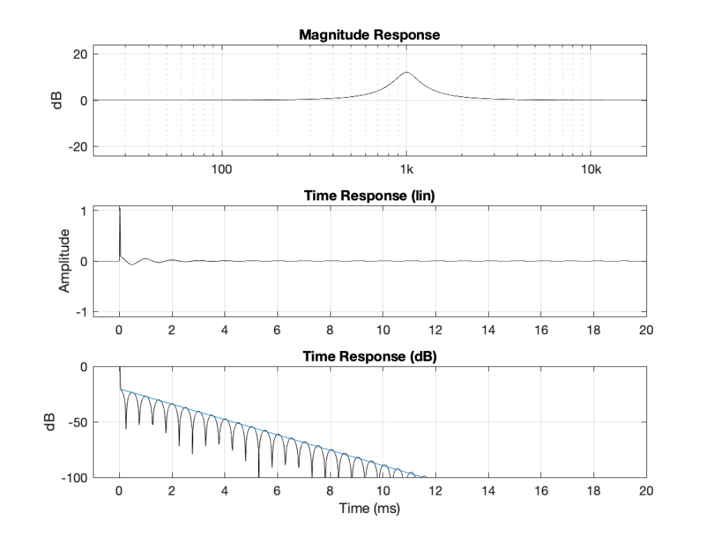
I could plot lots more of these so that you start to see a pattern, but I’ll jump to the punch lines and you can use the plots above to check that things make sense.
If I have a filter that is using a definition of Q = Fc / BW (where BW is the distance between the -3 dB points down from the maximum), then:
- Changing the gain does not change the rate of the decay (all least, as long as it’s a boost, according to what we’ve seen so far…)
- Changing the Q will change the slope of the decay inversely proportionally if we’re measuring the slope in dB/sec. For example, if I multiply the Q by 2, the ringing decays twice as slowly. If I multiply the Q by 10, the ringing will take 10 times longer to decay to the same level.
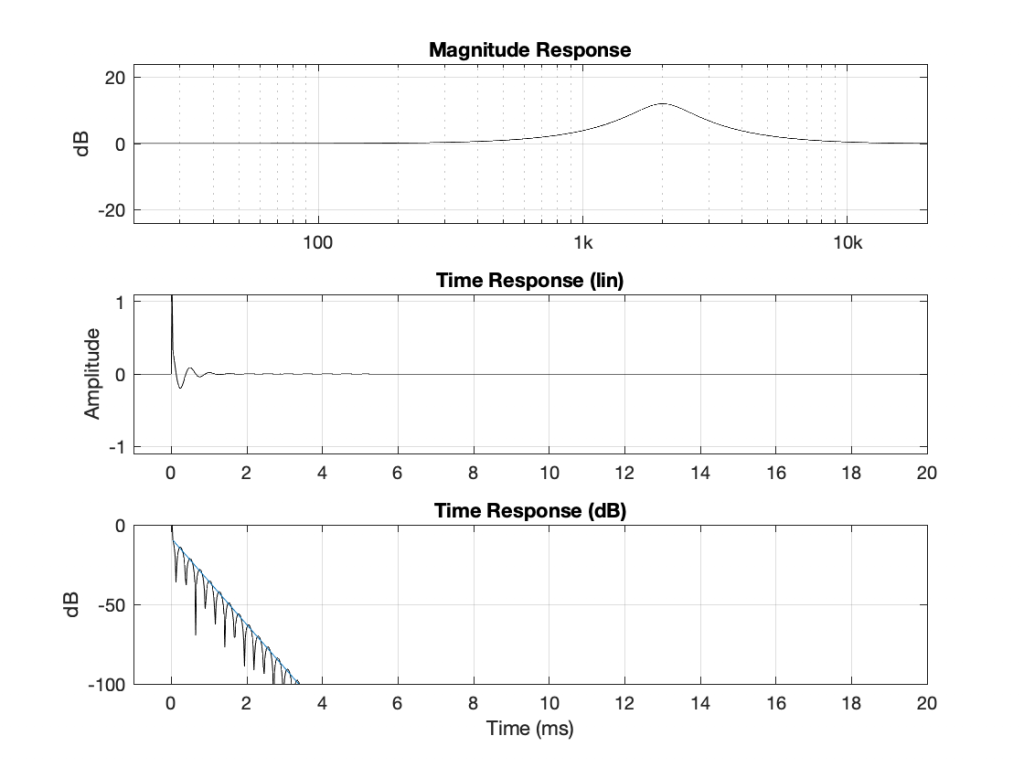
- Changing the frequency will change the slope of the decay proportionally if we’re measuring the slope in dB/sec. For example, if I multiply the frequency by 2, the ringing will decay twice as fast.
Let’s talk about the last of these first, since it’s the easiest to understand conceptually. In the plots above, I’m showing the time in seconds. So, the higher the frequency, the more cycles I’m showing in the same plot. However, if I were plotting time in cycles of the cosine wave instead, the slope would be the same regardless of frequency.
In other words, the level of the ringing decays by the same amount per number of cycles of the cosine wave.
This is why, if you count the number of “bumps” in the dB plots in Figure 2 and 5, you’ll see that they are the same number. It takes about 12 cycles to get down to -100 dB, but the shorter the cycles (because the frequency is higher) the faster you get there when measuring in seconds. If the X-axis were not “Time in milliseconds”, but “Time in periods of the centre frequency” instead, then the slopes would be identical in Figures 2 and 5.