Let’s put together a couple of things that were said in the last postings, which should help to support each other:
A peak or a dip filter is created by adding a bandpass filter to a throughput, as shown in Figure 1.
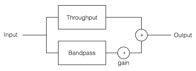
To change from peak to dip, you switch the polarity of the bandpass portion by making the “gain” negative instead of positive. (In other words, you subtract the bandpass from the throughput instead of adding it). To change the gain of the peak/dip filter, you change the gain of the bandpass portion. To change the Q of the peak/dip, you change the Q of the bandpass.
We also saw at the end of Part 3 that changing the gain does not change the rate of the decay.
This should all come together nicely to make sense for the first of the three points. For example, since the bandpass portion is the part that’s ringing, and since changing the gain of the peak (or dip) is just a matter of changing the gain applied to the bandpass portion, then there is no reason why the decay rate of the ringing should change. It will start at a higher or lower level, but its decay slope will be the same.
Q vs Time
We also saw at the end of Part 3 that changing the Q will change the slope of the decay inversely proportionally, but that changing the frequency will change the slope of the decay proportionally.
There is a nice little rule-of-thumb that’s used by electrical engineers for measuring the Q of a filter. Let’s say that you can’t (or couldn’t be bothered to take the time to) measure the frequency or magnitude response, and you want to figure out the Q based on the time response only, you can calculate this by looking at its impulse response.
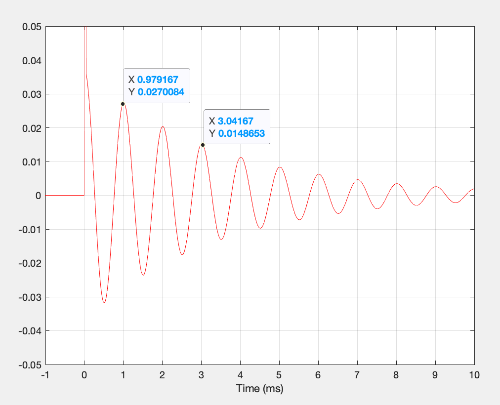
For example, Figure 2 shows the initial part of the impulse response of an unknown filter. I’ve highlighted two points that are reasonably close to the tops of two of the cosine wave cycles. I picked the first one (on the left) and then noted its Y value (Y = 0.027). Then I found a top of another wave that was as close to half that value as I could find. You can see there that it’s 2 cycles later, where Y = 0.0149.
So, you multiply the number of cycles it takes to drop by 50% (in this example, 2 cycles) and multiply that by 4.53, which results in a value of about 9. This is a good estimate of the Q of the filter (which is actually 10, if I measure it using the -3 dB points in the magnitude response).
If you’d like to read the long version of this, check out this page.
Note that it doesn’t matter which cycle I chose to get the first value, since the rate of decay is the same through the entire time response of the filter. In other words, if I chose the 3rd cycle to do the first measurement, I would have found that the 5th cycle is about 50% lower because it’s also 2 cycles later.
It also doesn’t matter whether we’re talking about peaks or dips, since, as we already know, from a perspective of the individual building blocks of the filter, these are the same thing.
So what?
Of course, most normal people aren’t measuring the time response of filters to calculate the Q. However, this piece of information is good from the opposite perspective: if you know the Q of the filter, you can figure out how fast it’s decaying. For example, a filter with a Q of 2 will take 2 / 4.53 = 0.44 cycles to decay by 50% (or 6 dB). If you know the frequency, then you can then translate that into a decay rate per seconds, because the period in seconds (the total time of one cycle of the wave) = 1 / Fc.
So, if that filter with a Q of 2 has an Fc of 100 Hz, then the period is 1/100 = 0.01 sec, and therefore it will decay by 6 dB (50%) in 0.44 cycles * 0.01 sec/cycle = 0.0044 sec or 4.4 ms.
If the Fc of the filter is 5 kHz, then the the period is 1/5000 = 0.0002 sec, and therefore it will decay by 5 dB in 0.0002 * 0.44 = 0.000088 sec = 88 µsec. (This is roughly equivalent to 2 samples at 48 kHz.)
Another good thing to remember is that Q = Fc / BW where BW is the bandwidth of the response measured between the two -3 dB points. This means, for example, that if Q = 1, then Fc = BW, therefore the bandwidth is about 1 octave. If Q = 2, then the bandwidth is about 1/2 of an octave, if Q = 12 then the bandwidth is about 1 semitone (1/12th of an octave), and so on.