#69 in a series of articles about the technology behind Bang & Olufsen loudspeakers
#68 in a series of articles about the technology behind Bang & Olufsen loudspeakers
#65 in a series of articles about the technology behind Bang & Olufsen loudspeakers
Although active Beam Width Control is a feature that was first released with the BeoLab 90 in November of 2015, the question of loudspeaker directivity has been a primary concern in Bang & Olufsen’s acoustics research and development for decades.
As a primer, for a history of loudspeaker directivity at B&O, please read the article in the book downloadable at this site. You can read about the directivity in the BeoLab 5 here, or about the development Beam Width Control in BeoLab 90 here and here.
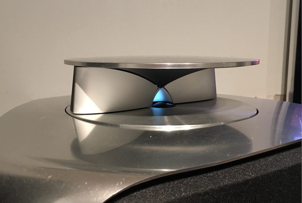
Bang & Olufsen has just released its second loudspeaker with Beam Width Control – the BeoLab 50. This loudspeaker borrows some techniques from the BeoLab 90, and introduces a new method of controlling horizontal directivity: a moveable Acoustic Lens.
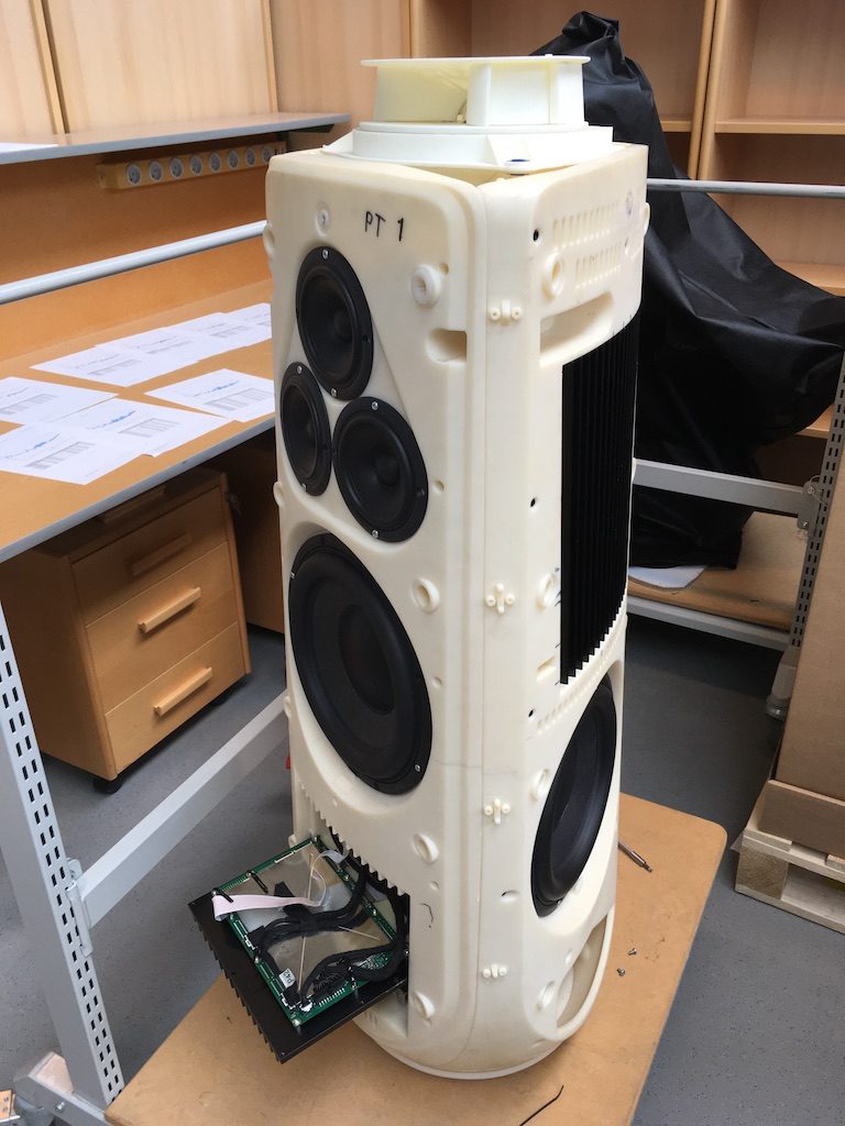
The three woofers and three midrange drivers of the BeoLab 50 (seen above in Figure 1) are each driven by its own amplifier, DAC and signal processing chain. This allows us to create a custom digital filter for each driver that allows us to control not only its magnitude response, but its behaviour both in time and phase (vs. frequency). This means that, just as in the BeoLab 90, the drivers can either cancel each other’s signals, or work together, in different directions radiating outwards from the loudspeaker. This means that, by manipulating the filters in the DSP (the Digital Signal Processing) chain, the loudspeaker can either produce a narrow or a wide beam of sound in the horizontal plane, according to the preferences of the listener.
You’ll see that there is only one tweeter, and it is placed in an Acoustic Lens that is somewhat similar to the one that was first used in the BeoLab 5 in 2002. However, BeoLab 50’s Acoustic Lens is considerably different in a couple of respects.
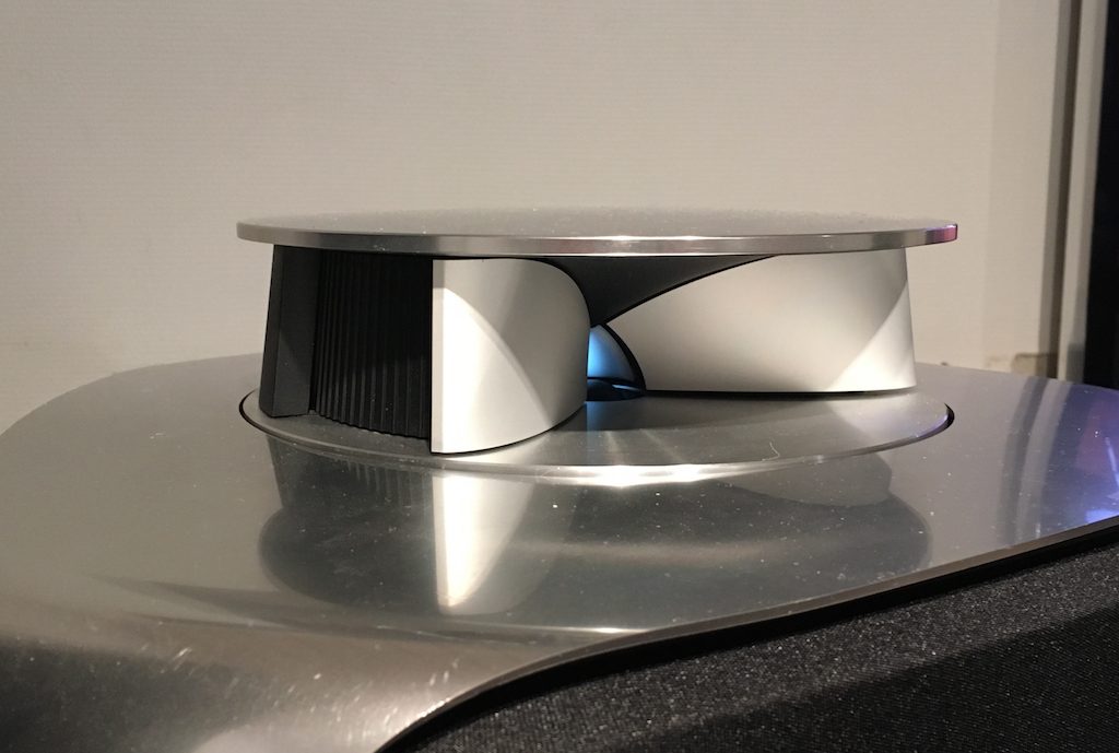
Firstly, the geometry of the Lens has been completely re-engineered, resulting in a significant improvement in its behaviour over the frequency range of the loudspeaker driver. One of the obvious results of this change is its diameter – it’s much larger than the lens on the tweeter of the BeoLab 5. In addition, if you were to slice the BeoLab 50 Lens vertically, you will see that the shape of the curve has changed as well.
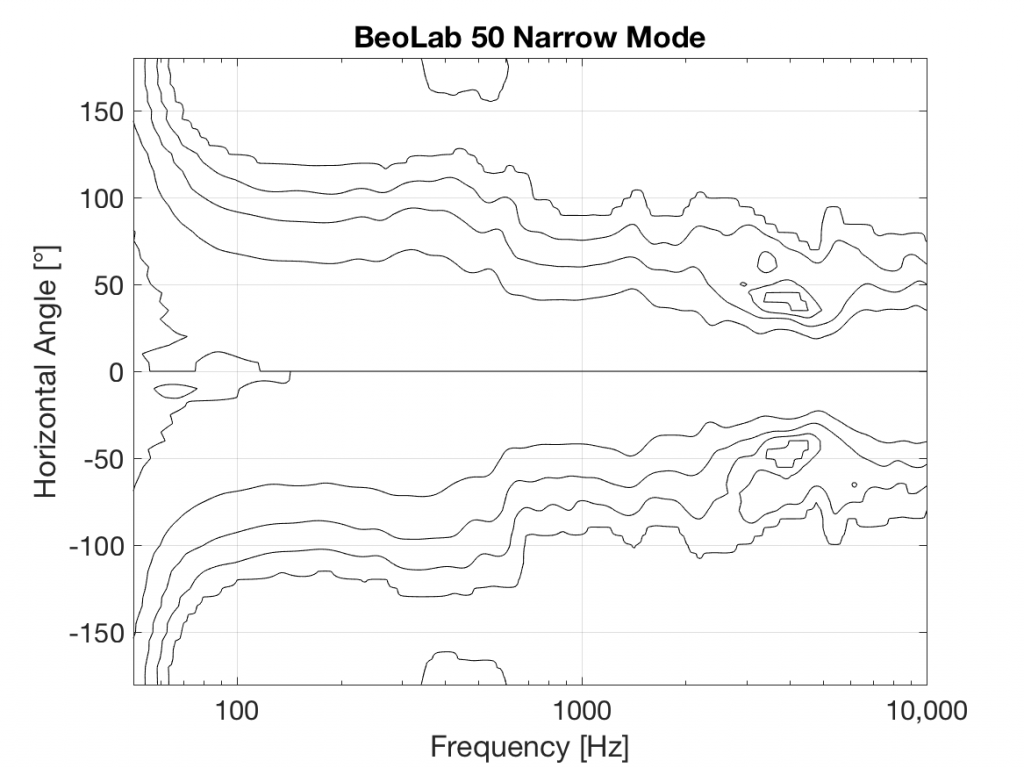
However, the Acoustic Lens was originally designed to ensure that the horizontal width of sound radiating from a tweeter was not only more like itself over a wider frequency range – but that it was also quite wide when compared to a conventional tweeter. So what’s an Acoustic Lens doing on a loudspeaker that can also be used in a Narrow mode? Well, another update to the Acoustic Lens is the movable “cheeks” on either side of the tweeter. These can be angled to a more narrow position that focuses the beam width of the tweeter to match the width of the midrange drivers.
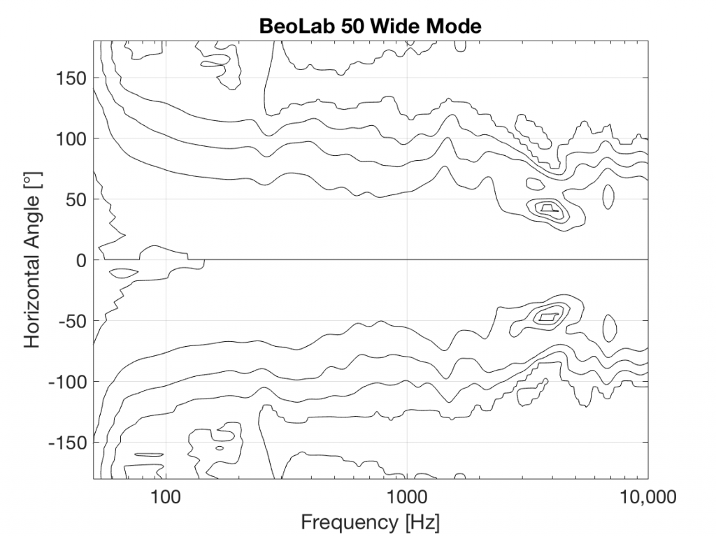
In Wide Mode, the sides of the lens open up to produce a wider radiation pattern, just as in the original Acoustic Lens.
So, the BeoLab 50 provides a selectable Beam Width, but does so not only “merely” by changing filters in the DSP, but also with moving mechanical components.
Of course, changing the geometry of the Lens not only alters the directivity, but it changes the magnitude response of the tweeter as well – even in a free field (a theoretical, infinitely large room that is free of reflections). As a result, it was necessary to have a different tuning of the signal sent to the tweeter in order to compensate for that difference and ensure that the overall “sound” of the BeoLab 50 does not change when switching between the two beam widths. This is similar to what is done in the Active Room Compensation, where a different filter is required to compensate for the room’s acoustical behaviour for each beam width. This is because, at least as far as the room is concerned, changing the beam width changes how the loudspeaker couples to the room at different frequencies.
In the last posting, I talked about the effects of a bandpass filter on the probability density function (PDF) of an audio signal. This left the open issue of other filter types. So, below is the continuation of the discussion…
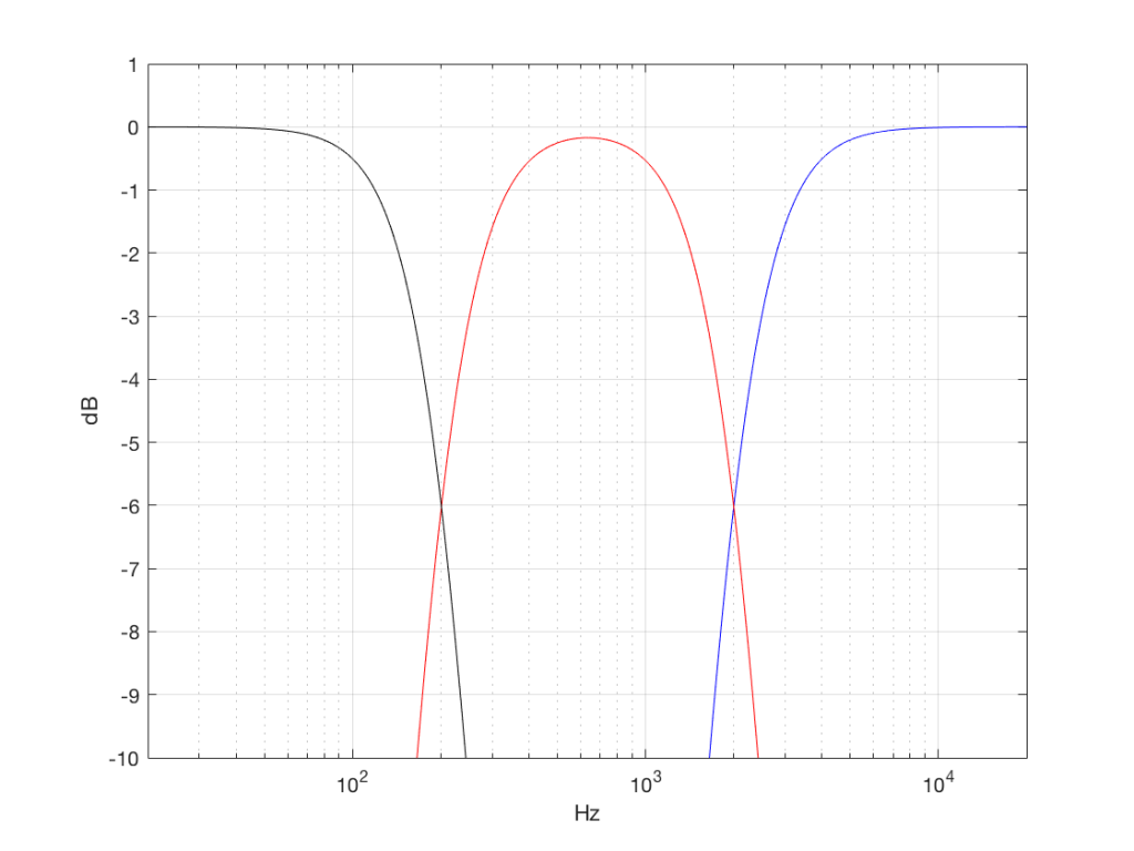
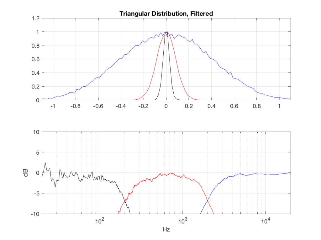
I made noise signals (length 2^16 samples, fs=2^16) with different PDFs, and filtered them as if I were building a three-way loudspeaker with a 4th order Linkwitz-Riley crossover (without including the compensation for the natural responses of the drivers). The crossover frequencies were 200 Hz and 2 kHz (which are just representative, arbitrary values).
So, the filter magnitude responses looked like Figure 1.
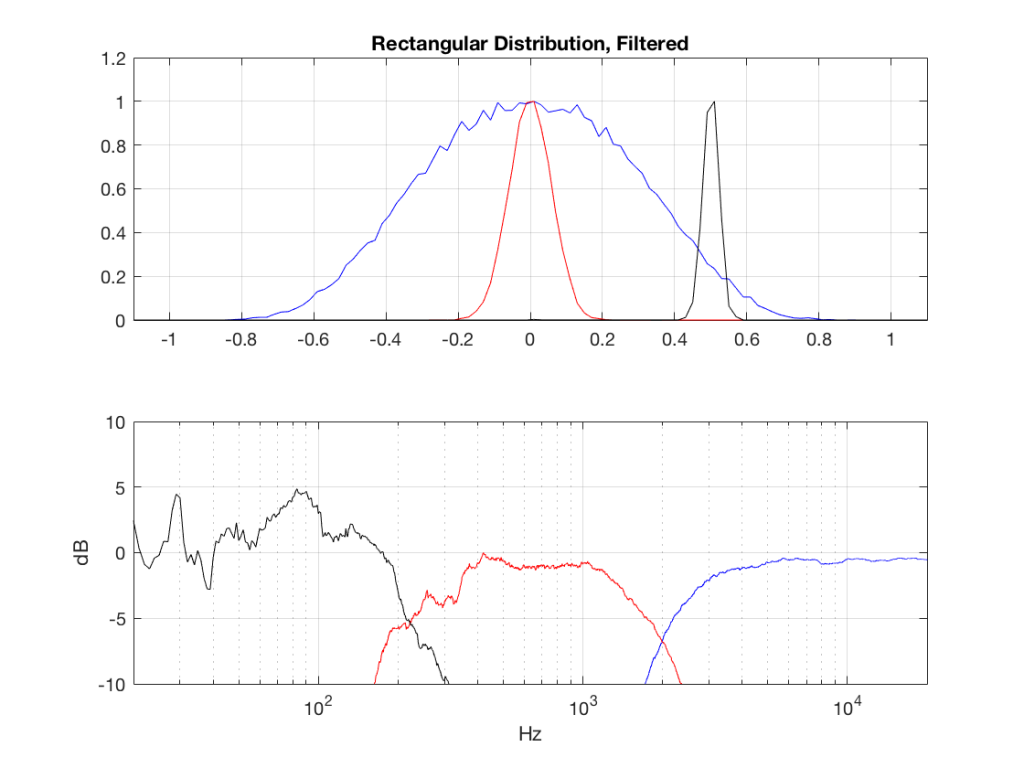
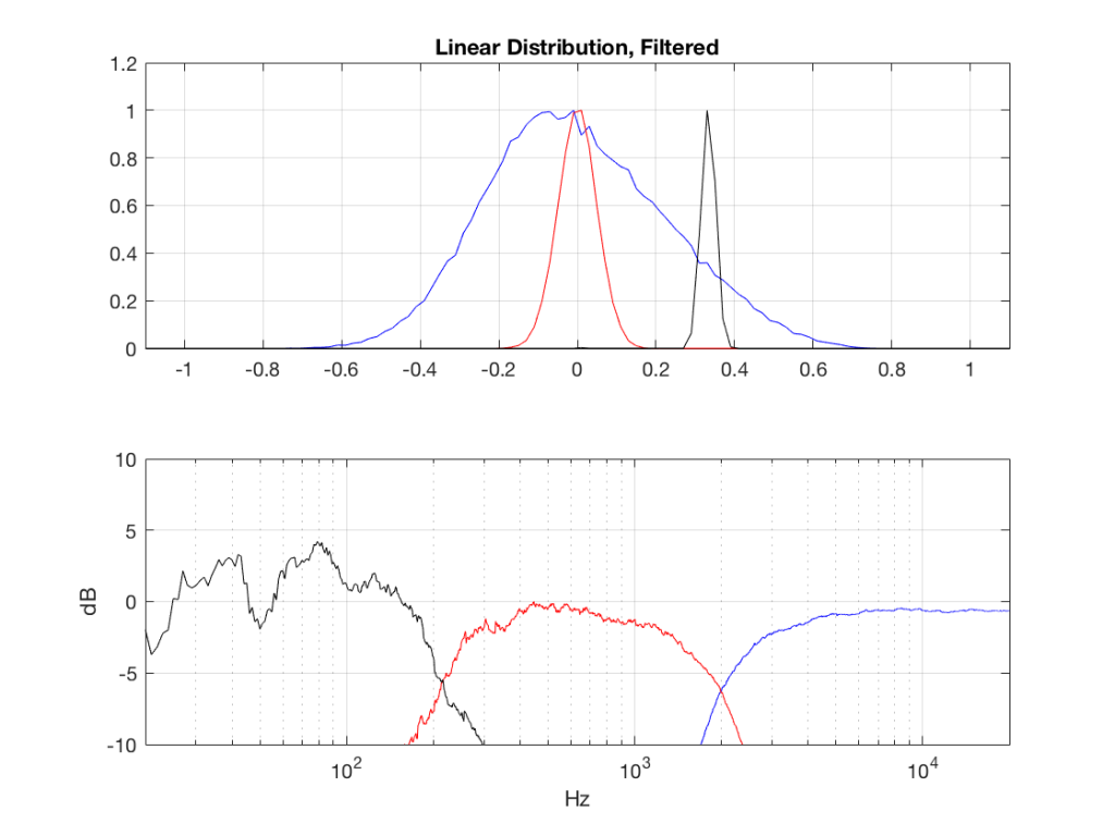
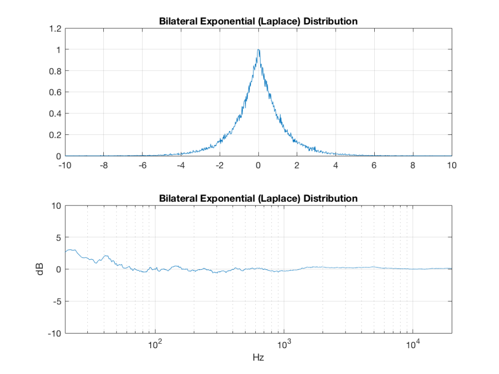
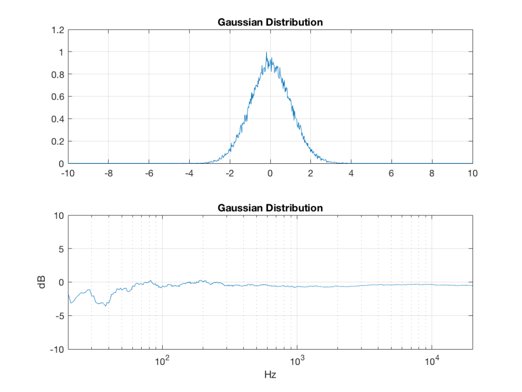
The resulting effects on the probability distribution functions are shown below. (Check the last posting for plots of the PDFs of the full-band signals – however note that I made new noise signals, so the magnitude responses won’t match directly.)
The magnitude responses shown in the plots below have been 1/3-octave smoothed – otherwise they look really noisy.
This posting has a Part 1 that you’ll find here and a Part 2 that you’ll find here.
In a previous posting, I showed some plots that displayed the probability density functions (or PDF) of a number of commercial audio recordings. (If you are new to the concept of a probability density function, then you might want to at least have a look at that posting before reading further…)
I’ve been doing a little more work on this subject, with some possible implications on how to interpret those plots. Or, perhaps more specifically, with some possible implications on possible conclusions to be drawn from those plots.
To start, let’s create some noise with a desired PDF, without imposing any frequency limitations on the signal.
To do this, I’ve ported equations from “Computer Music: Synthesis, Composition, and Performance” by Charles Dodge and Thomas A. Jerse, Schirmer Books, New York (1985) to Matlab. That code is shown below in italics, in case you might want to use it. (No promises are made regarding the code quality… However, I will say that I’ve written the code to be easily understandable, rather than efficient – so don’t make fun of me.) I’ve made the length of the noise samples 2^16 because I like that number. (Actually, it’s for other reasons involving plotting the results of an FFT, and my own laziness regarding frequency scaling – but that’s my business.)
uniform = rand(2^16, 1);
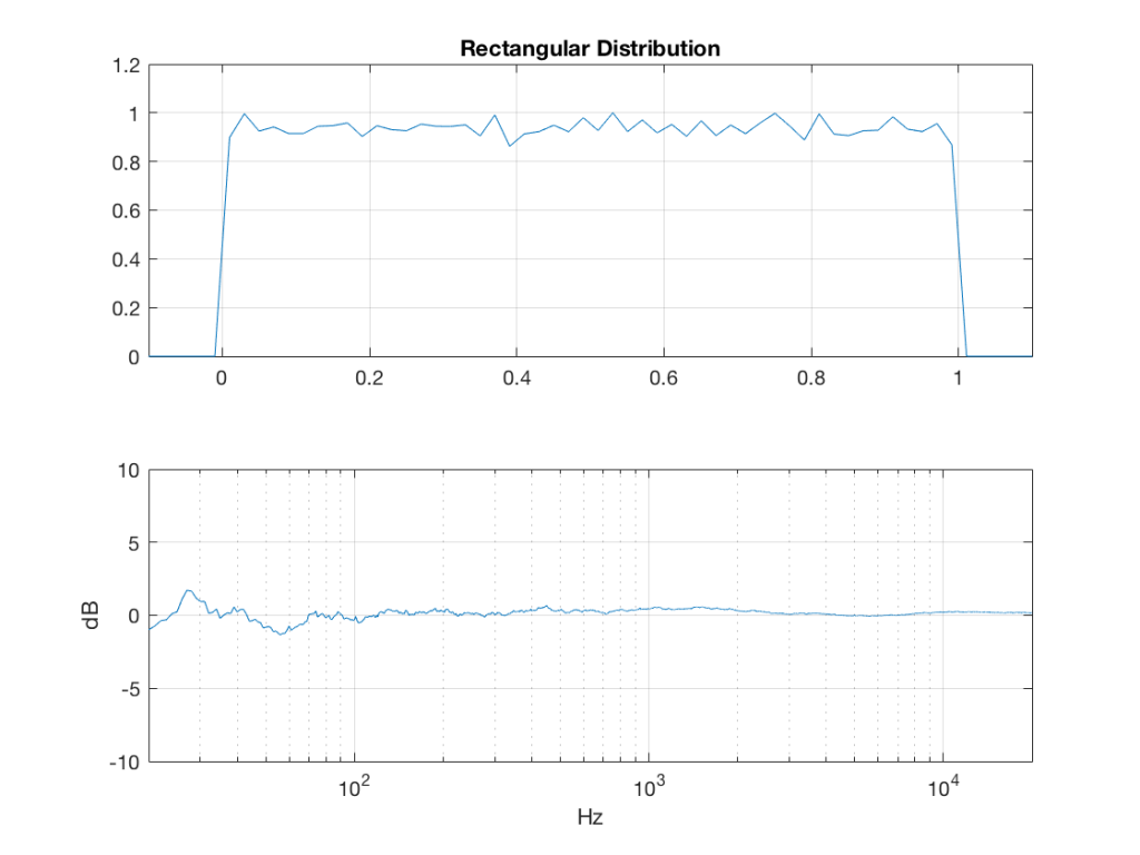
Of course, as you can see in the plots in Figure 1, the signal is not “perfectly” rectangular, nor is it “perfectly” flat. This is because it’s noise. If I ran exactly the same code again, the result would be different, but also neither perfectly rectangular nor flat. Of course, if I ran the code repeatedly, and averaged the results, the average would become “better” and “better”.
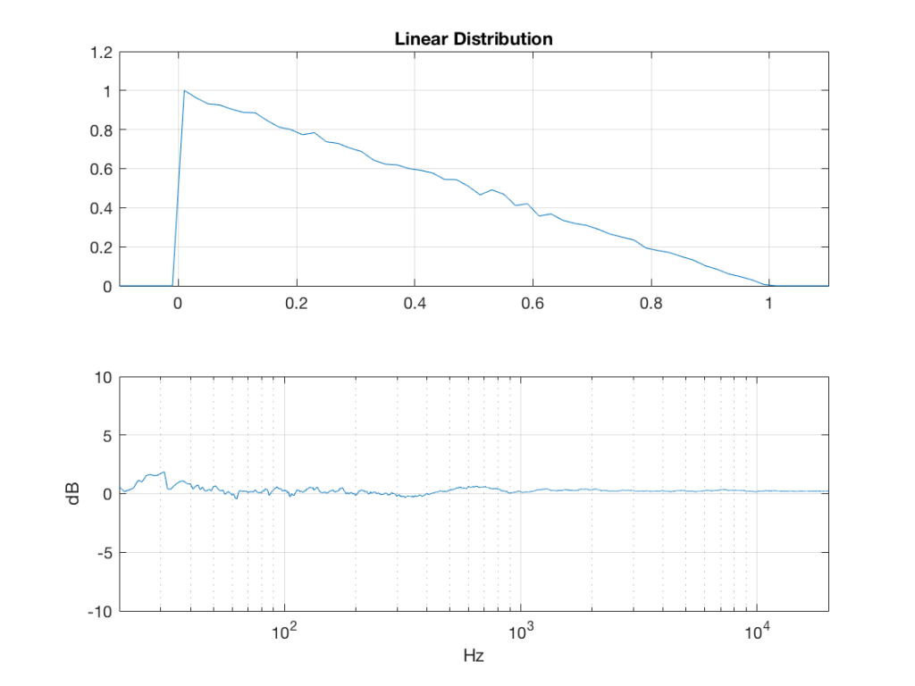
linear_temp_1 = rand(2^16, 1);
linear_temp_2 = rand(2^16, 1);
temp_indices = find(linear_temp_1 < linear_temp_2);
linear = linear_temp_2;
linear(temp_indices) = linear_temp_1(temp_indices);
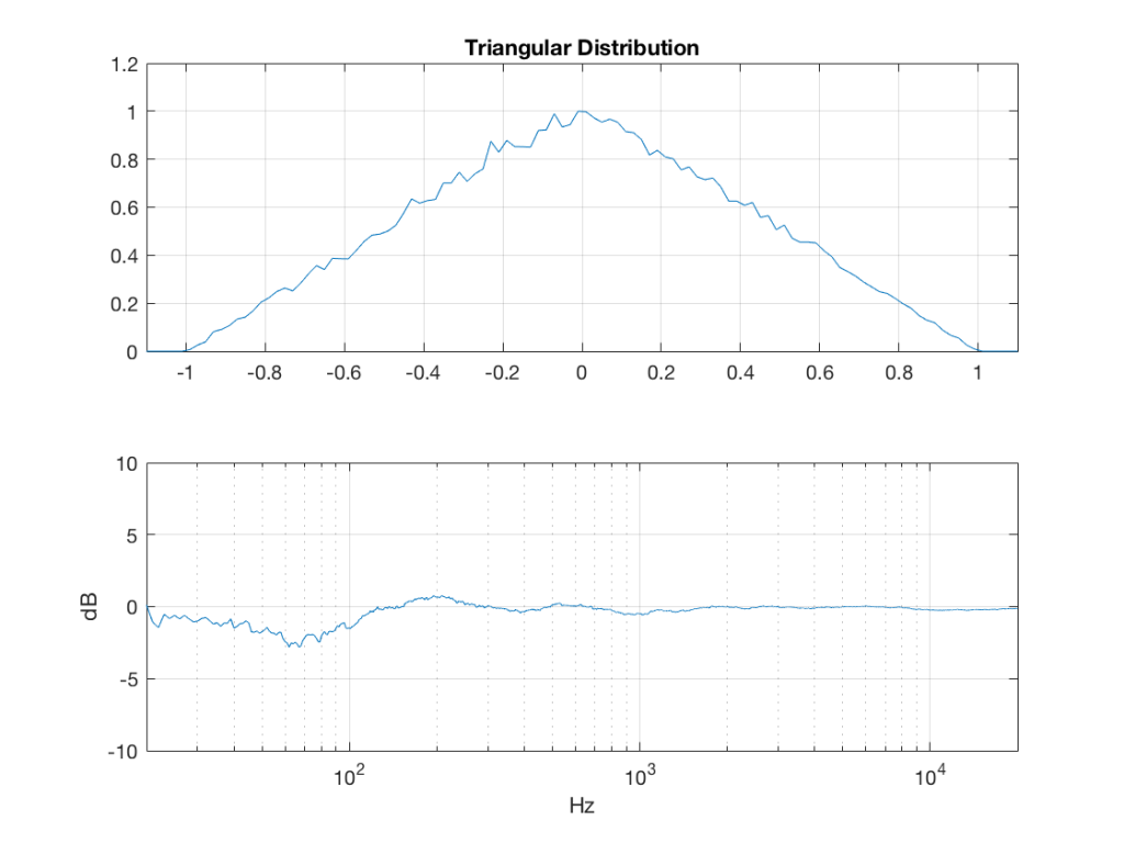
triangular = rand(2^16, 1) – rand(2^16, 1);
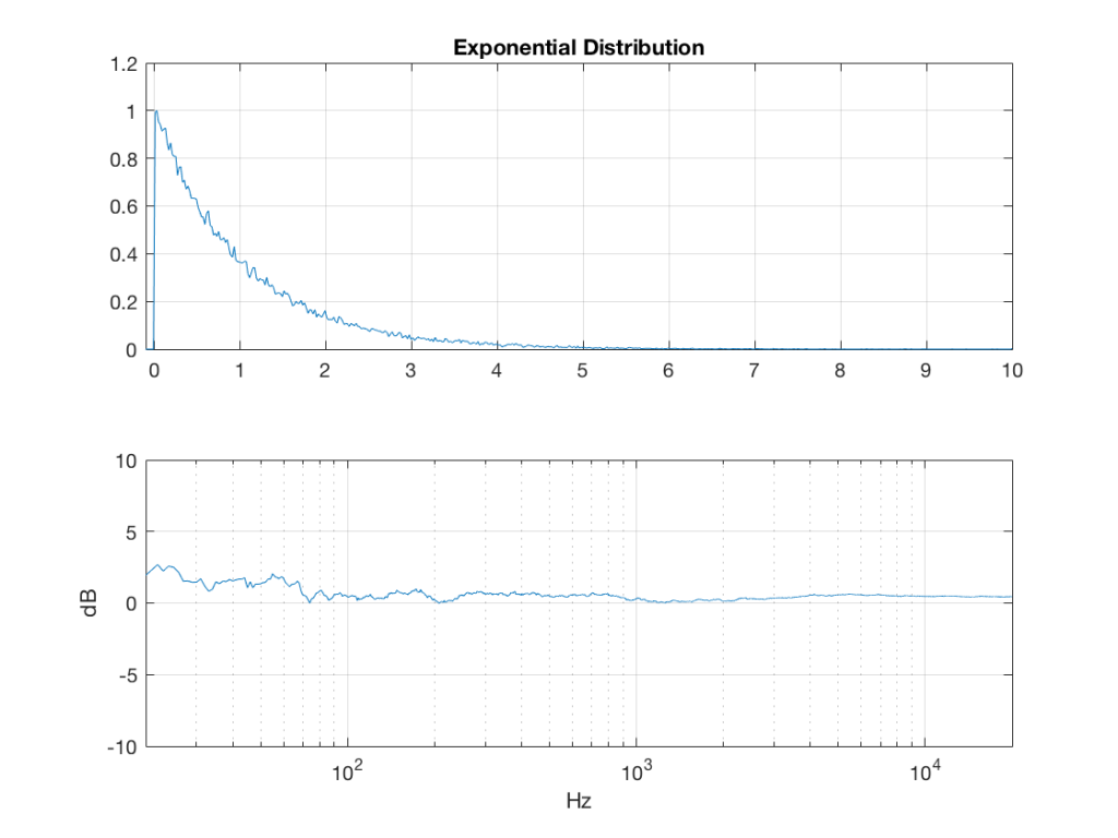
lambda = 1; % lambda must be greater than 0
exponential_temp = rand(2^16, 1) / lambda;
if any(exponential_temp == 0) % ensure that no values of exponential_temp are 0
error(‘Please try again…’)
end
exponential = -log(exponential_temp);
lambda = 1; % must be greater than 0
bilex_temp = 2 * rand(2^16, 1);
% check that no values of bilex_temp are 0 or 2
if any(bilex_temp == 0)
error(‘Please try again…’)
end
bilex_lessthan1 = find(bilex_temp <= 1);
bilex(bilex_lessthan1, 1) = log(bilex_temp(bilex_lessthan1)) / lambda;
bilex_greaterthan1 = find(bilex_temp > 1);
bilex_temp(bilex_greaterthan1) = 2 – bilex_temp(bilex_greaterthan1);
bilex(bilex_greaterthan1, 1) = -log(bilex_temp(bilex_greaterthan1)) / lambda;
sigma = 1;
xmu = 0; % offset
n = 100; % number of random number vectors used to create final vector (more is better)
xnover = n/2;
sc = 1/sqrt(n/12);
total = sum(rand(2^16, n), 2);
gaussian = sigma * sc * (total – xnover) + xmu;
Of course, if you are using Matlab, there is an easier way to get a noise signal with a Gaussian PDF, and that is to use the randn() function.
What happens to the probability distribution of the signals if we band-limit them? For example, let’s take the signals that were plotted above, and put them through two sets of two second-order Butterworth filters in series, one set producing a high-pass filter at 200 Hz and the other resulting in a low-pass filter at 2 kHz .(This is the same as if we were making a mid-range signal in a 4th-order Linkwitz-Riley crossover, assuming that our midrange drivers had flat magnitude responses far beyond our crossover frequencies, and therefore required no correction in the crossover…)
What happens to our PDF’s as a result of the band limiting? Let’s see…
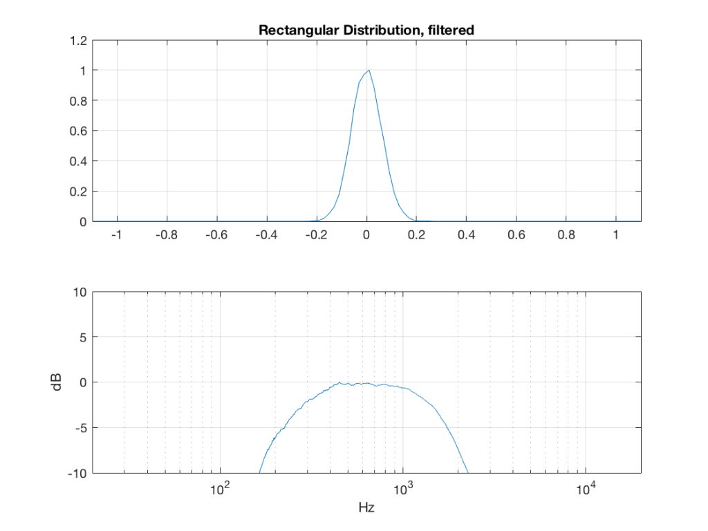
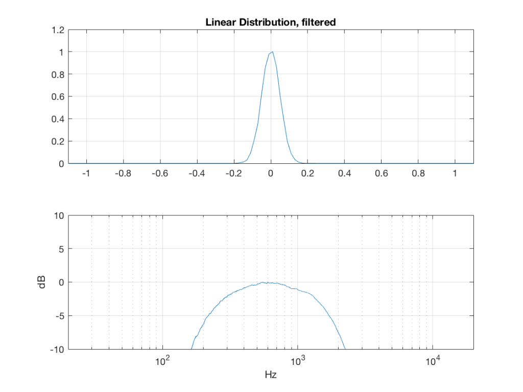
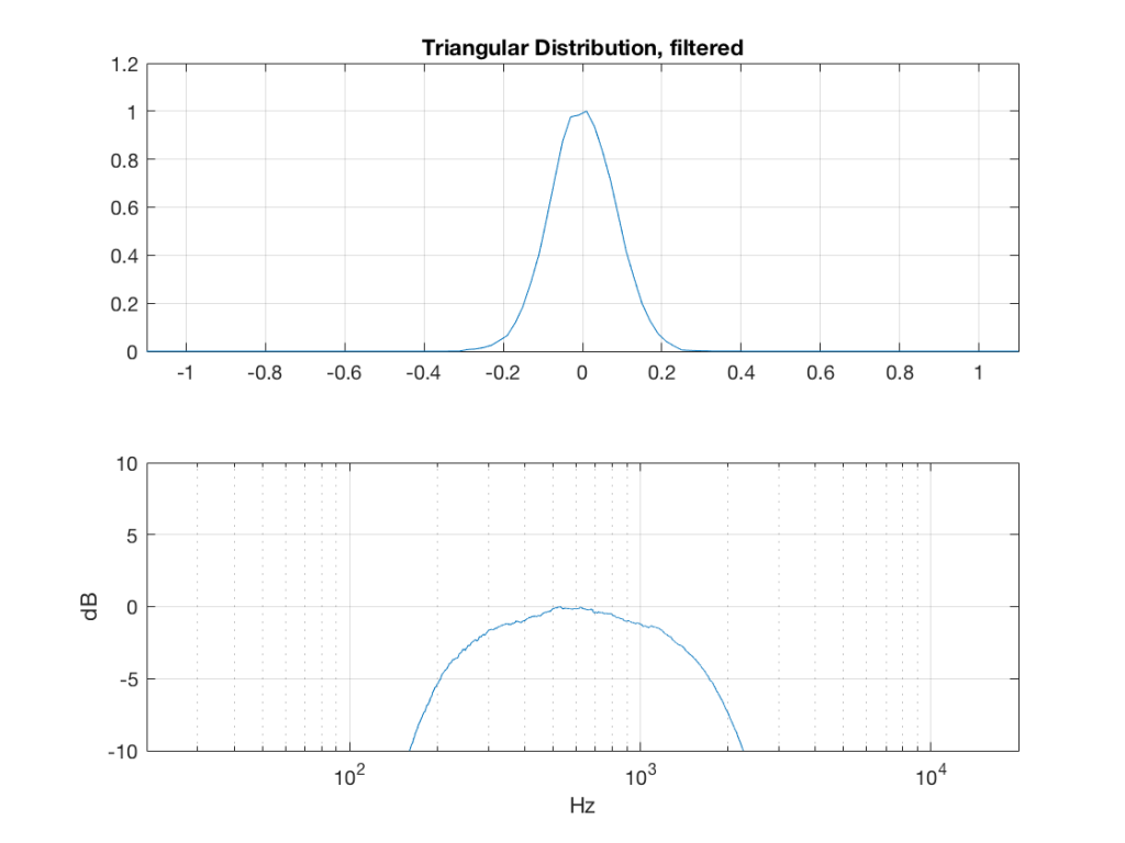
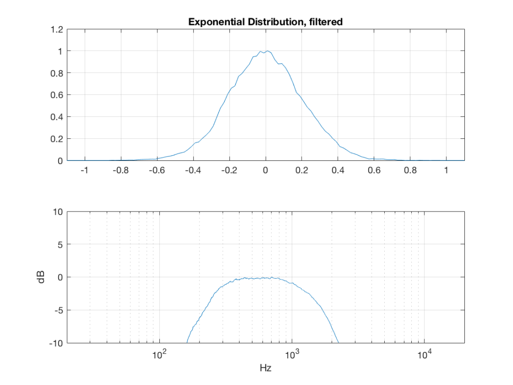
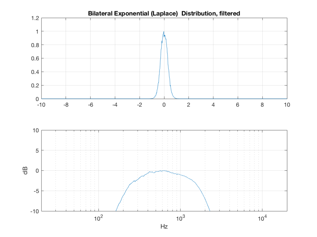
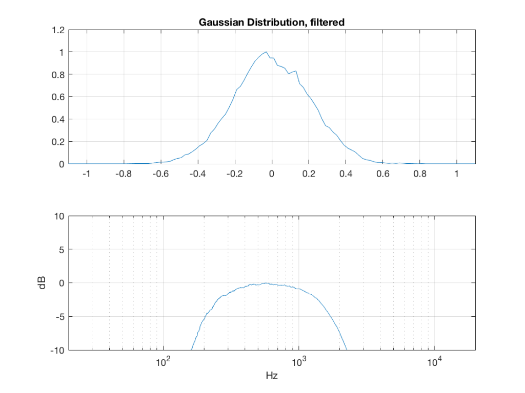
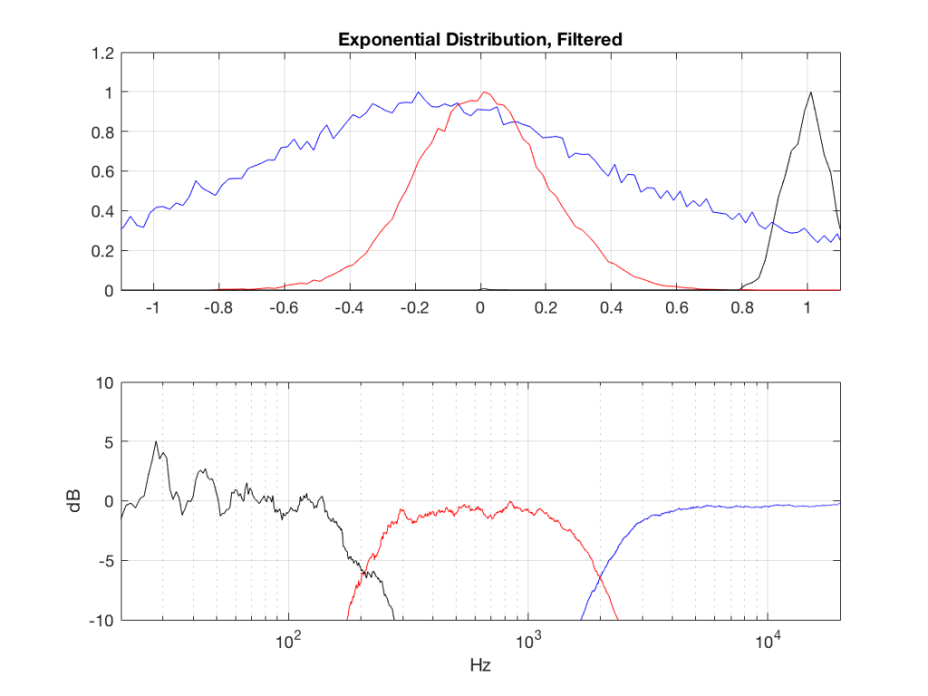
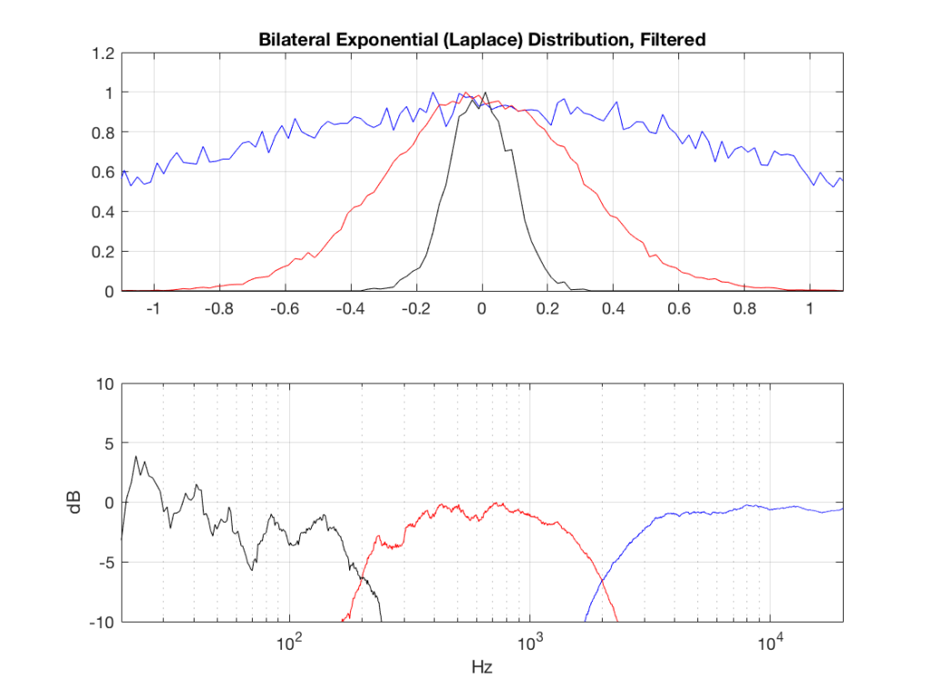
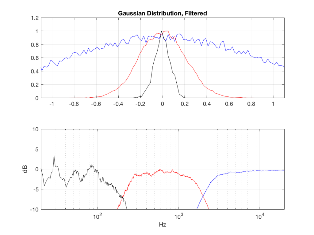
So, what we can see in Figures 7 through 12 (inclusive) is that, regardless of the original PDF of the signal, if you band-limit it, the result has a Gaussian distribution.
And yes, I tried other bandwidths and filter slopes. The result, generally speaking, is the same.
One part of this effect is a little obvious. The high-pass filter (in this case, at 200 Hz) removes the DC component, which makes all of the PDF’s symmetrical around the 0 line.
However, the “punch line” is that, regardless of the distribution of the signal coming into your system (and that can be quite different from song to song as I showed in this posting) the PDF of the signal after band-limiting (say, being sent to your loudspeaker drivers) will be Gaussian-ish.
And, before you ask, “what if you had only put in a high-pass or a low-pass filter?” – that answer is coming in a later posting…
This posting has a Part 1 that you’ll find here, and a Part 3 that you’ll find here.
#64 in a series of articles about the technology behind Bang & Olufsen products
Stephen Colbert once said that George W. Bush was a man of conviction. He believed the same thing on Wednesday that he believed on Monday, no matter what happened on Tuesday….
Often people ask me questions about sound quality. In “the old days”, it was something like “which is better, analogue or digital?” Later, it became “which is better, MP3 or Ogg Vorbis (or something else)?”. These days, it’s something like “which streaming service has the best quality?” or “Is high-resolution audio really worth it?” Or, it’s a more general question like “what loudspeaker (or headphones) would you recommend?”
My answer to these questions is always the same. It’s a combination of “it depends….” and “whatever I tell you today, it might be different tomorrow…”Something that is true on Monday may not still be true on Wednesday…
Recently, during a discussion about something else, I told someone that many, if not most, mobile devices will clip (and therefore) distort a signal if you try to boost it (e.g. with a “bass boost” or a “pop” setting instead of playing the signals “flat”), but they won’t if you cut. Therefore, on a mobile device, it’s smarter to cut than to boost a signal.
I made that statement based on some past measurements that were done that showed that, if you put a 0 dB FS signal at a low frequency (say, 80 Hz) on different mobile devices, and turned the “bass boost” (or equivalent, such as a “pop” or “rock” setting) on, the signal would be often be clipped, and therefore it would increase the level of distortion – sometimes quite dramatically. The measurements also showed that this was independent of volume setting. So, turning down the level didn’t help – it just made things quieter, but maintained the same THD value. This is likely because the processing in such devices & software was done (a) before the volume control and (b) in a fixed-point system that does not have a carefully-managed headroom.
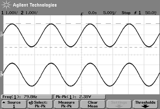
So, just to be sure that this was still true on newer devices and software, I did a couple of quick measurements. I put a logartihmically-swept sine wave with a level of 0 dB FS and a frequency range of 20 Hz to 2 kHz on a current mobile audio device with a minijack headphone output. With the output volume at maximum and the EQ set to “OFF” or “FLAT”, I recorded the output and did a little analysis.
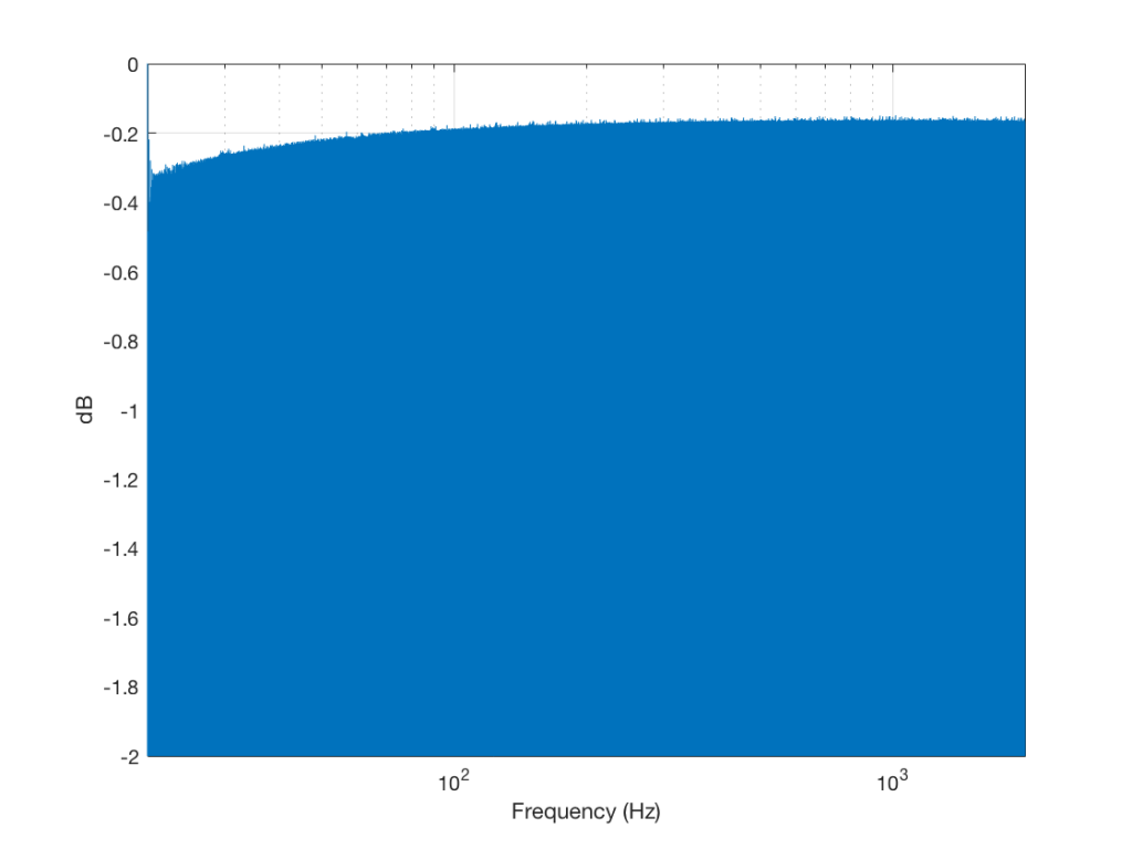
Although Figure 4 is a plot of the time-domain output of the system (in other words, I’m just plotting 20*log10(abs(signal)), it can be read as a frequency response plot (which is why I’ve labelled it that way on the x-axis). Actually, though, I have to be explicit and say that we’re actually looking at the absolute value of the signal itself, and the y-axis is labelled as the frequency at the time of the signal coming in.
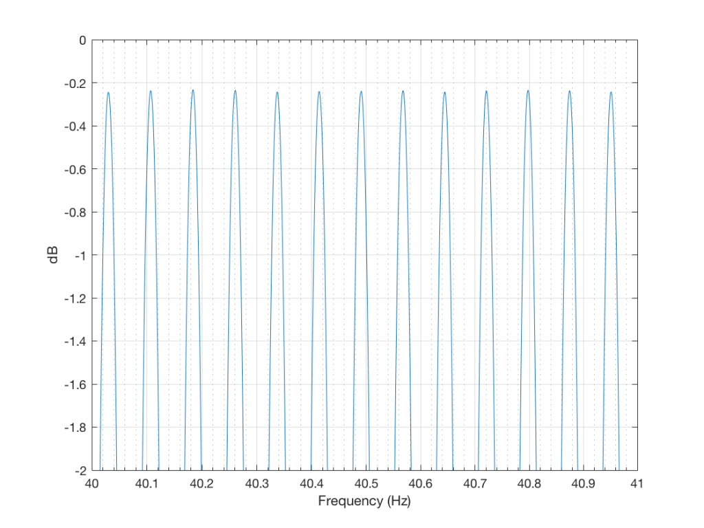
If we zoom in on the signal, we get the plot shown in Figure 5.
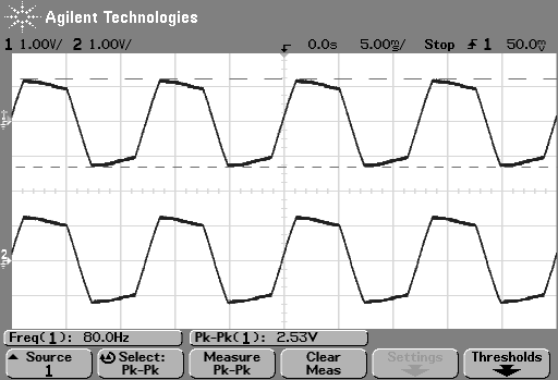
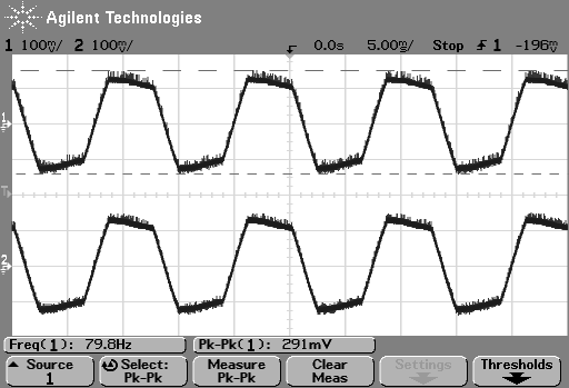
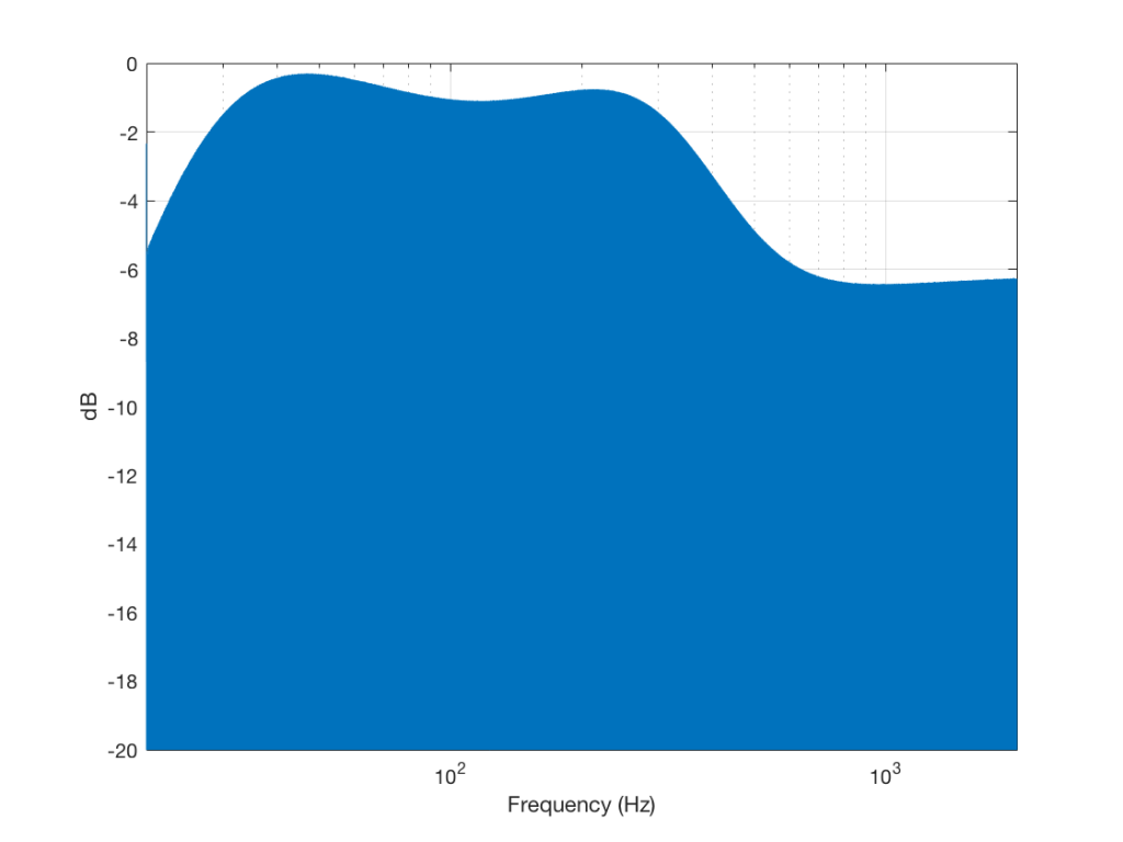
Then I turned the bass boost setting to “ON” and repeated the recording, without changing anything else. The result is shown in Figure 6.
Zooming in on the same 40 Hz region, we see the following:
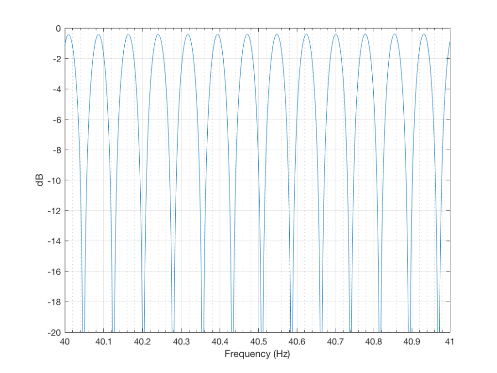
So, as can be seen in those plots, the clipping problem that used to be quite obvious in some mobile devices has been corrected on this newer device due to a difference in the way the signal processing is implemented in the software.
However, as can be seen in Figure 6, this solution to the problem was to drop the midrange and treble by about 6 dB. (It’s also interesting that we lose almost 6 dB at 20 Hz when we think that we are boosting the “bass” – but that’s another discussion…) This might be considered to be a smart solution, since the listener can just turn up the level to compensate for the loss, if they wish. However, it does mean that, on this particular device, with this particular software version, if you do turn on the “bass boost” function, you’ll lose about 6 dB from your maximum level (which is equivalent to 4 times the sound power) in the midrange and high frequency regions (say, from about 600 Hz and up, give or take…). So, distortion has been traded for a lower maximum output level in the comparison between these two devices and software versions, two years apart.
So, generally speaking, it seems that I have fallen victim to exactly the problem that I often warn people to avoid. I believed the same thing on Wednesday that I believed on Monday… Then again, I know for certain that there are many people who are still walking around with the same distorting software / device that I complained in the “old days” (those first set of measurements are only 2 years old…). And, if you’re concerned about maximum output levels, the “new” solution might also not be optimal for your preferences.
So, it seems that “it depends” is still the safest answer…