#38 in a series of articles about the technology behind Bang & Olufsen loudspeakers
In the last posting, I talked about a little experiment we did that made us realise that control of a loudspeaker’s directivity (or more simply “beam width”) would be a useful parameter in the hands of a listener. And, in a previous article, I talked a little about why that is probably true. This week, let’s get our hands dirty and talk about how Beam Width Control can be accomplished.
Part 1: What is sound?
Okay – we’re really getting back to basics, but it won’t take long. I promise. In order to get to where we’re headed, we have to have a fairly intuitive grasp of what sound is. At a basic level, sound is a change in air pressure over time. Today’s atmospheric (or barometric) pressure is about 100 kiloPascals (give or take). That pressure can be thought of as a measure of the average distances between the air molecules in the room you’re sitting in. It is also important to note that (unless you’re very unlucky and very uncomfortable) the pressure inside your head is roughly the same as the pressure outside your head (otherwise, you’d probably be talking about going to visit a doctor…). The important thing about this is that this means that the pressure that is exerted on the outside of your eardrum (by the air molecules sitting next to it in your ear canal) is almost identical to the pressure that it exerted on the inside of your eardrum (the part that’s inside your head). Since the two sides are being pressed with the same force, then the eardrum stays where it should.
However, if we momentarily change the air pressure outside your head, then you eardrum will be pushed inwards (if the pressure is higher on the outside of your head) or pulled outwards (if the pressure is lower). This small, momentary change in pressure can be caused by many things, but one of those things is, for example, a woofer getting pushed out of its cabinet (thus making a “high pressure” where the air molecules are squeezed closer together than normal) or pulled into its cabinet (thus making a “low pressure” and pulling the air molecules apart).
So, the woofer pushes out of the cabinet, squeezes the air molecules together which push your eardrum into your head which does a bunch of things that result in you hearing a sound like a kick drum.
Part 2: Frequency and wavelength
Take a loudspeaker into your back yard and play a tone with the same pitch as a “Concert A” (the note you use to tune a violin – or, at least, the note violinists use to start tuning a violin…). This note has a frequency of 440 Hz, which means that your loudspeaker will be moving from its resting position, outwards, back, inwards, and back to the resting position (a full cycle of the tone) 440 times every second. This also means that your eardrum is getting pushed inwards and and pulled outwards 440 times every second.
Now, turn off the loudspeaker and walk 344 m away. When you get there, turn on the tone again. You’ll notice that you don’t hear it right away because sound travels pretty slowly in air. In fact, it will take almost exactly one second from the time you turn on the loudspeaker to the time the sound reaches you, since the speed of sound is 344 m/s (you’re 344 m away, so it takes one second for the sound to get to you).
If, at the instant you start to hear the tone, you were able to freeze time – or at least freeze the air molecules between you and the loudspeaker, you’d see something interesting (at least, I think it’s interesting). The instant you hear the start of the tone (the first cycle), the 441st cycle is starting to be generated by the loudspeaker (because it’s producing 440 cycles per second, and it’s been one second since it started playing the tone). This means that, in your frozen-time-world, there are 440 high and low pressure zones “floating” in the 344 m of air between you and the loudspeaker. Given this information, we can calculate how long the length of one wave is (better known as the “wavelength” of the tone). It’s 344 m divided by 440 cycles per second = 78.2 cm.
So, this means that there are 78.2 cm between each high pressure “bump” in the air. This also means that there is half that distance (39.1 cm) between adjacent high and low pressure zones in the air.
Part 3: Interference
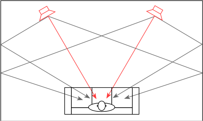
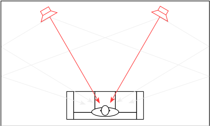
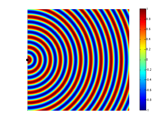
Now let’s take a case where we have two woofers. We’ll put them side by side and we’ll send the same 440 Hz tone to them. So, when one woofer goes out, the other one does as well. This means that each one creates a high pressure in front of it. If you’re exactly the same distance from the two woofers, then those two high pressures add together and you get an even higher pressure at the listening position (assuming that there are no reflecting surfaces nearby). This is called constructive interference. This happens when you have two loudspeaker drivers that are either the same distance from the listening position as in Figure 2 or in exactly the same location (which is not possible), as in Figure 3.


If we change the wiring to the woofers so that they are in opposite polarity, then something different happens. Now, when one woofer goes outwards, the other goes inwards by the same amount. This means that one creates a high pressure in front of it while the other creates a low pressure of the same magnitude. If you’re exactly the same distance from the two woofers, then those two pressures (one high and one low) arrive at the same time and add together, so you get a perfect cancellation at the listening position (assuming that there are no reflecting surfaces nearby). This is called destructive interference. This is shown in Figure 4 and 5.


However, an important thing about what I just said was that you are the same distance from the two woofers. What if you’re not? Let’s say, for example, that you’ve changed your angle to the “front” of the loudspeaker (which has two loudspeaker drivers). This means that you’re closer to one driver than the other. The result is that, although the two drivers are playing the same signal at the same time, your difference in distance causes their individual signals to have different phases at the listening position – possibly even a completely opposite polarity – as is shown in Figure 5.

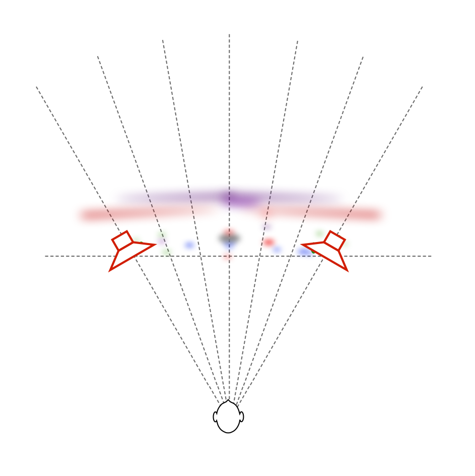
If you consider Figure 2 and Figure 5 together (they’re really two different views of the same situation, since both loudspeakers are playing the same signal simultaneously) and you include all other listening positions, then you get Figure 6. As you can see there, there is no sound (again, indicated by the greenish colour which means no change in pressure) at the angle shown in Figure 5.
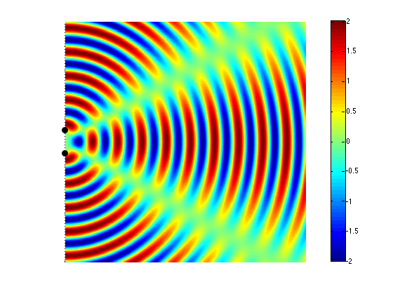
So, Figure 6 shows that, for a position directly in front of the sound sources (to the right of the black dots, in the figure), the result is identical to that in Figure 3 – the two sources add together perfectly if you’re the same distance from them. However, if you start to move away from that line, so that you’re closer to one sound source than the other, then, at some angle, you will get a high pressure from the upper sound source at the same time as you get the previous low pressure from the lower source (because it’s farther away from you, and therefore a bit late in time…) This high+low = nothing, and you hear no sound.
Another, slightly more nuanced way to do this is to not just change the polarity of one of the sound sources, but to alter its phase instead. This is a little like applying a delay to the signal sent to the driver, but it’s a delay that is specific to the frequency that we’re considering. An example of this is shown in Figure 7.

This means that, by changing the phase instead of the polarity of the drivers, I can “steer” the direction of the beam and the “null” (the area where the sound is cancelled out)
It should be noted that, at a different separation of the drivers (more accurately stated: at a different relationship between the wavelength of the signal and the distance between the drivers) , the behaviour would be different. For example, look at Figure 8 which shows the same situation as Figure 6 – the only difference is that the two sound sources are half the distance apart (but the wavelength of the signal has remained the same).

Part 4: Putting it together
So, at a very basic level (so far) we can determine which direction sound is radiated in based on a relationship between
- the wavelength of the signal it is producing (which is a function of its frequency)
- the distance between the sound sources (the loudspeaker drivers), and
- the polarity and/or the phase of the signals sent to the drivers.
All of the examples shown above assume that the two sound sources (the loudspeaker drivers) are playing at the same level, which is not necessarily the case – we can choose to play a given frequency at whatever level we want using a rather simple filter. So, by reducing the level of the “interfering” driver, we can choose how much the directivity of the radiated sound is affected.
In addition to this, all of the examples shown above assume that the sound sources are omnidirectional – that they radiate sound equally at all frequencies – which is not true in real life. In real life, a loudspeaker driver (like a tweeter or a woofer) has some natural directivity pattern. This pattern is different at different frequencies and is influenced by the physical shapes of the driver and the enclosure it’s mounted on.
So, let’s start putting this together.
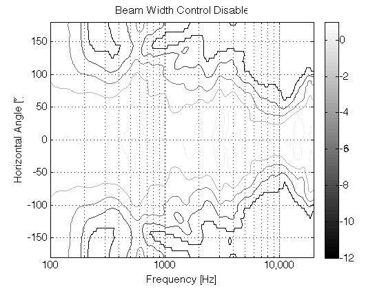
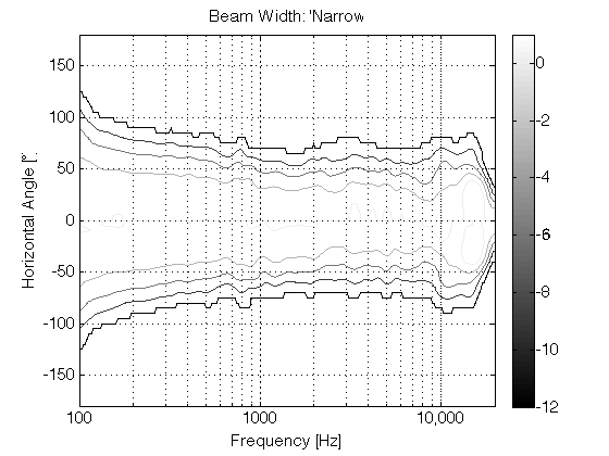
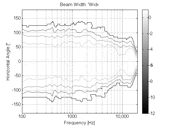
If I take a loudspeaker driver – say, a midrange unit – and I mount it on the front of a loudspeaker enclosure and measure its directivity pattern (the geeky term for the width of its sound beam) across its frequency range and beyond I’ll see something like this:

As you can see in that plot, in its low frequency range (the red line on the left), the midrange driver is radiating sound with a wide beam – not completely omnidirectional, but very wide. In its high frequency region (around the right-hand red line) (but still not high enough to be re-routed to the tweeter) the midrange is “beaming” – meaning that the beam is getting too narrow. Our goal is to somehow make the beam widths at these frequency bands (and the ones in between) more alike. So, we want to reduce the width of the beam in the low frequencies and increase the width of the beam in the high frequencies. How can we do this? We’ll use more midrange drivers!
Let’s take two more midrange drivers (one on either side of the “front” or “main” one) and use those to control the beam width. In the lower frequencies, we’ll send a signal to the two side drivers that cancel the energy radiated to the sides of the loudspeaker – this reduces the width of the beam compared to using the front midrange by itself. At higher frequencies, we’ll send a signal to the two side drivers that add to the signal from the front driver to make the width of the beam wider. At a frequency in the middle, we don’t have to do anything, since the width of the beam from the front driver is okay by itself, so at that frequency, we don’t send anything to the adjacent drivers.
“Okay”, I hear you cry, “that’s fine for the beam width looking from the point of view of the front driver, but what happens as I come around towards the rear of the loudspeaker?” Excellent question! As you come around the rear of the loudspeaker, you won’t get much contribution from the front midrange, so the closest “side” midrange driver is the “main” driver in that direction. And, as we saw in the previous paragraph, the signal coming out of that driver is pretty strange (because we intentionally made it strange using the filters – it’s in opposite polarity in its low end, it doesn’t produce anything in its midrange, and it’s quiet, but has a “correct” polarity in its high end). So, we’ll need to put in more midrange drivers to compensate again and clean up the signal heading towards the rear of the loudspeaker. (What we’re doing here is basically the same as we did before, we’re using the “rear” drivers to ensure that all frequencies heading in one rearward direction are equally loud – so we make the “rear” drivers do whatever they have to do at whatever frequency bands they have to do it in to make this true.)
“Okay”, I hear you cry, “that’s fine for the beam width looking from the point of view of the rear of the loudspeaker, but what happens as we go back towards the front of the loudspeaker? Won’t the signals from the rear-facing drivers screw up the signal going forwards?” Excellent question! The answer is “yes”. So, this means that after the signal from the rear-facing midrange drivers is applied (which compensate for the side-facing midrange drivers which compensate for the front facing midrange driver) then we have to go back to the front and find out the effects of the compensation of the compensation on the “original” signal and compensate for that – so we start in a loop where we are compensating for the compensation for the for the compensation for the compensation for the… Well, you get the idea…
The total result is a careful balancing act where some things are known or given:
- the frequency range of the music being played through a given loudspeaker driver (this is limited by the crossover)
- the natural directivity patterns of the loudspeaker drivers on the loudspeaker enclosure within that frequency range
- the locations of the loudspeaker drivers in three-dimensional space
- the orientations of the loudspeaker drivers in three-dimensional space (in other words, which way they’re pointing)
Note that these last two have been calculated and optimised based on a combination of the natural directivity patterns of the loudspeaker drivers and the desired beam widths we want to make available.
As a result each individual loudspeaker driver gets its own customised filter that controls
- the level of the signal at any given frequency
- the phase (which includes delay and polarity – sort of…) of the signal at any given frequency

By controlling the individual output levels and phases of each loudspeaker driver at each frequency it produces, we can change the overall level of the combined signals from all the loudspeaker drivers in a given direction. If we want to be loud at 0º (on-axis) and 20 dB quieter at 90º (to the side), we just apply the filters to all of the drivers to make that happen. If we want the loudspeaker to be only 10 dB down at 90º, then this just means changing to a different set of filters. This can be done independently at different frequencies – with the end goal to make all frequencies behave more similarly, as I talked about in this posting and this posting.
Also, since the filters are merely settings of the DSP (the digital signal processing “brain” of the loudspeaker), we can change the beam width of the loudspeaker merely by loading different filters – one for each loudspeaker driver in the system.
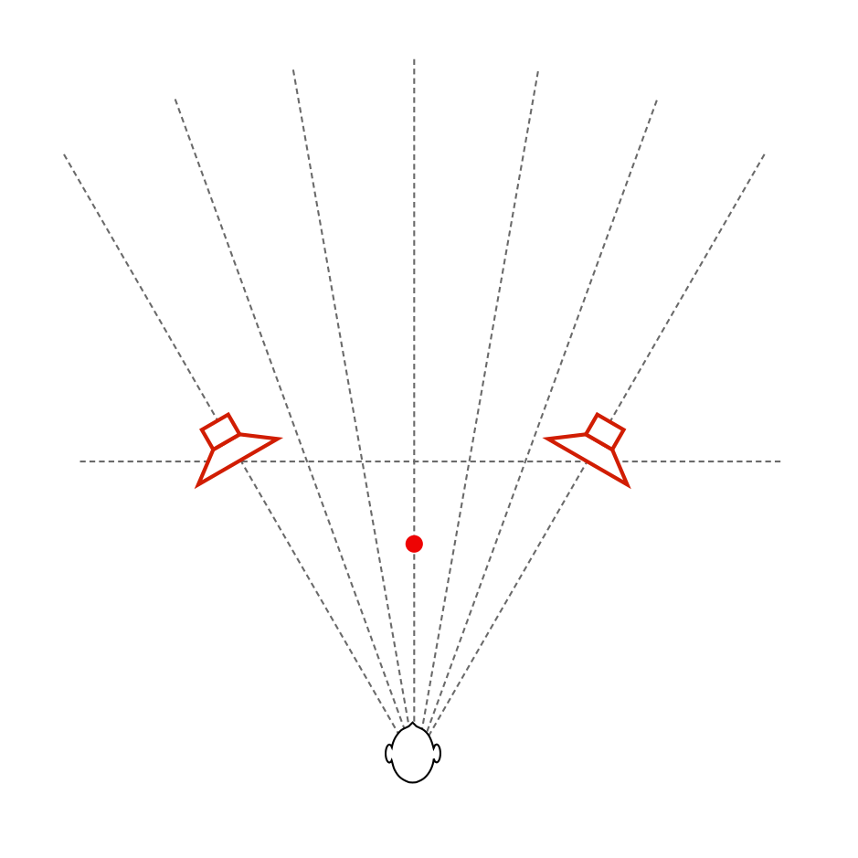
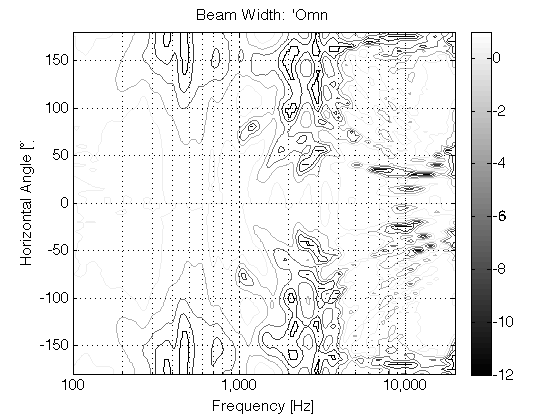
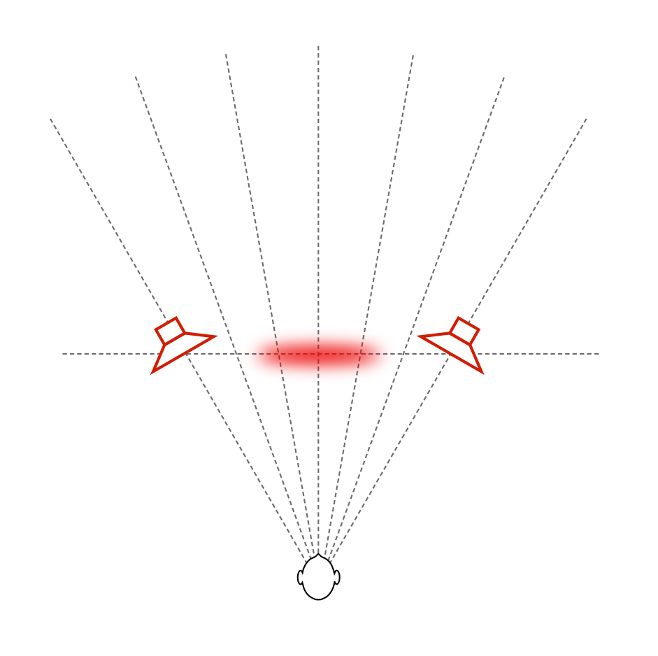
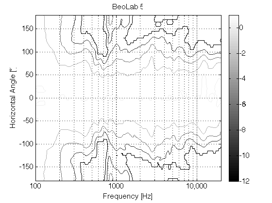
The end result is a loudspeaker that can play many different roles, as was shown in the different plots in this posting. In one mode, the beam width can be set to “narrow” for situations where you have one chair, and no friends and you want the ultimate “sweet spot” experience for an hour or two. In another mode, the beam width can be set to “wide”, resulting in a directivity that is very much like an improved version of the wide dispersion of the BeoLab 5. In yet another mode, the beam width can be set to “omni”, sending sound in all directions, making a kind of “party mode”.
Part 5: The “side” effect: Beam Direction Control
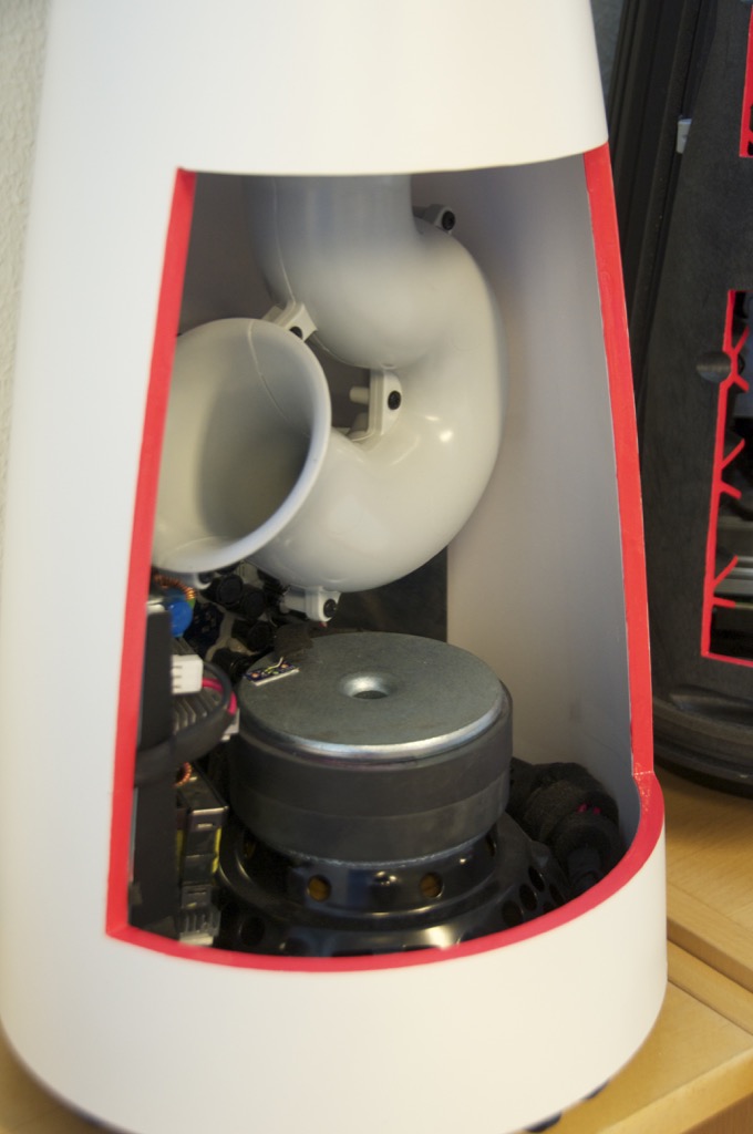
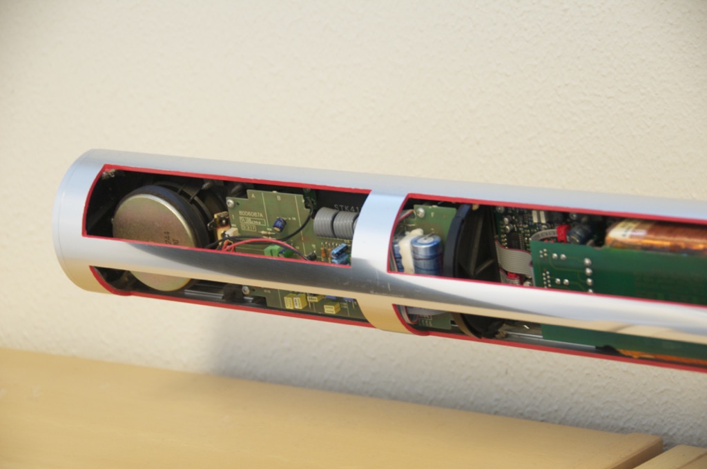
In order to be able to have a Beam Width Control, a loudspeaker must have a number of identical loudspeaker drivers. A collection of tweeters, midranges and woofers, some on the front, some on the sides and some to the rear of the loudspeaker. In addition, each of these drivers must have its own amplifier and DSP channel so that it is independently controllable by the system.
This means that, instead of using the drivers to merely control the width of the beam in the front of the loudspeaker, they can also be used somewhat differently. We could, instead, decide to “rotate” the sound, so that the “main” tweeter and midrange are the ones on the side (or even the rear) of the loudspeaker instead of the ones on the front. This means that, if you’re sitting in a location that is not directly in front of the loudspeakers (say, to the sides, or even behind), it could be possible to improve the sound quality by “rotating” the “on-axis” direction of the loudspeaker towards your listening position. This by-product of Beam Width Control is called Beam Direction Control.
P.S. Apologies for the pun…
For more information on Beam Width Control: