In this part, we’re going to do something a little weird.

We’ll start by making a minimum phase peaking filter that has Q of 2 and a gain of +6 dB. The response of that filter is shown in Figure 1.

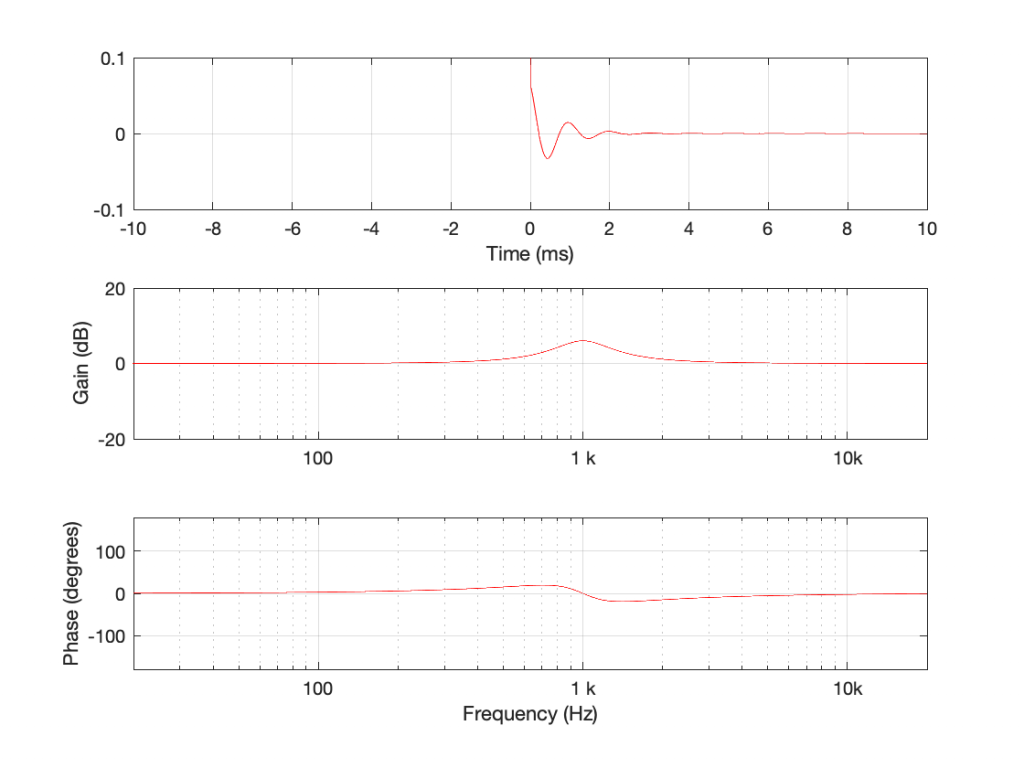
Almost everything in the plots above should look familiar. The one weird thing is that I’ve left out the data in the time response before T = 0 ms. That’s because the future doesn’t matter, since we’re talking about a non-causal filter, right?

What if I (for some reason) wanted to make a filter that had a desired magnitude response, but a flat phase response? Let’s say that you’re allergic to phase shifts or you belong to an ancient religious cult that thinks that phase shifts are against the order of nature. How would we create that filter?

One way to do it is to create a filter that has the same magnitude response as the one above, but with an opposite phase response so that the two cancel each other. But, how do we create a filter with the opposite phase response?

One trick for doing this is to ignore what I said earlier. Remember when I was being pedantic about how filters advance signals in phase BUT NOT TIME? What if you were to ignore that for a brief moment? Could we use that ignorance to an advantage?

For example, what would happen if we took the time response shown above and reversed it? All of the component frequencies are still there, at all the same relative amplitudes. So the Magnitude Response won’t change. But what happens to the phase response? The answer is this:

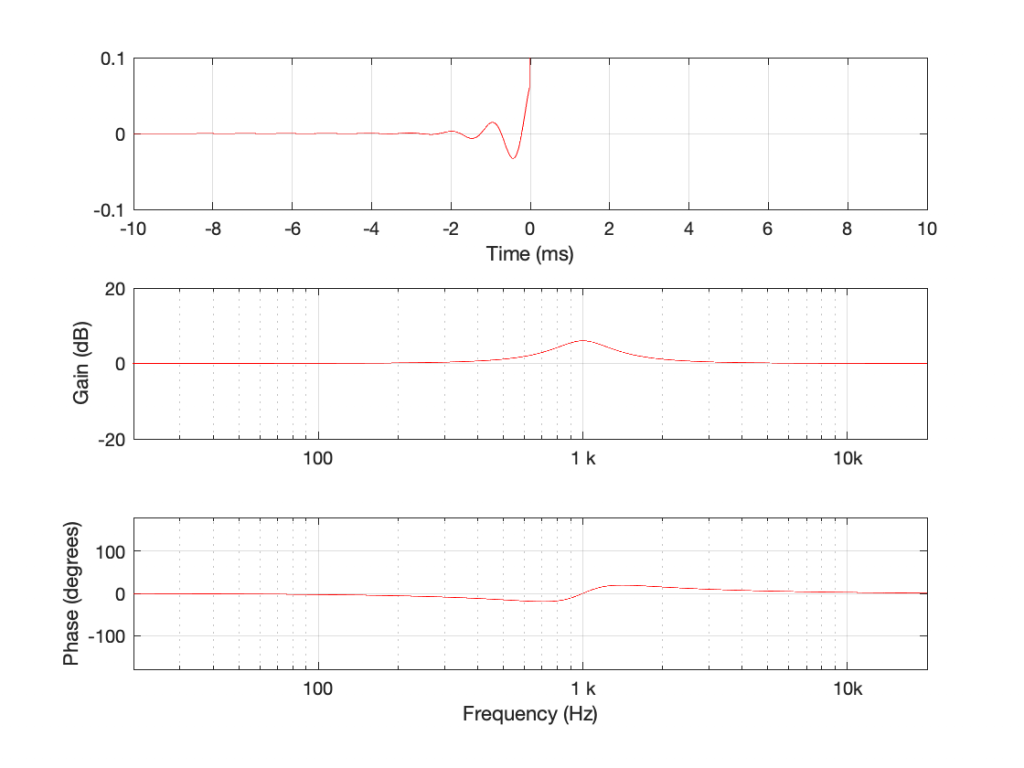
Now we have a weird filter that can only have an output based on future inputs (therefore it’s non-causal, and therefore not minimum-phase), with the same magnitude response as the one shown in Figure 1. But check out that phase response. It’s the inverse of the first filter.

So reversing time has the effect of flipping the polarity of the phase (not the polarity of the signal!) without modifying the magnitude response. What would have been a 45º phase shift (earlier) becomes a -45º phase shift (later).

So, if I were (conceptually – not really…) to put these two filters in series, feeding the output of one into the input of the other then their total magnitude responses would add (so I’d get a 12 dB boost instead of a 6 dB boost at 1 kHz) and their phase responses would cancel each other out. The end result would look like this:

By now, you’ve probably figured out that what we’re looking at here is a linear phase filter, since can be used to change the magnitude response of a signal without mucking up its phase response.

The catch with this way of implementing a linear phase filter is that it has to see into the future. Of course, in real life this is difficult, but there is a trick you can use to fake it.

If you look at the impulse response plot in Figure 1, you can see that the peak in the response is at Time = 0 ms. As you get later, moving away from that moment in time, the signal is quieter and quieter until it dies away to (almost) nothing. The problem is that ‘almost nothing’ is not the same as ‘nothing’. In fact, if we’re being pedantic, the ringing keeps going forever, which is why it’s called a filter with an Infinite Impulse Response – an IIR filter.

This also means that the same is true for the filter in Figure 2, but the ringing extends infinitely backwards in time.

However, our resolution in measuring and storing the amplitude is not infinite – when the signal is quiet enough, we run out of resolution (‘ticks’ on the ruler) – and when the signal gets that quiet, it effectively becomes the same as nothing.

So, if we decide on the level where ‘almost nothing’ is the same as ‘nothing’ (this is more-or-less up to us if we’re the ones designing the filter), then we can look at the filter’s response and decide when that signal level is reached (both forwards and backwards in time).

For example, with the extremely limited resolution of the plots that I’ve made above, we can decide that ‘nothing’ is what’s left when you get ±10 ms from the impulse peak. Of course, the resolution of the pixels on that plot is not even close to the resolution of the audio signal, so ‘nothing’ on our plot and ‘nothing’ for the audio signal are two different things – but the concept is the same.

Back to the Future

Let’s pretend for a moment that, for the impulse response in Figure 3, we decide that ±10 ms is the window of time we need to get to ‘nothing’. This means that we could implement this filter by sending audio into it, letting it pre-ring with an increasing amount until it hits the maximum peak 10 ms after the sound comes into it, then ringing for another 10 ms until it’s out.

This means that the latency (the delay time between the input and the output of the filter) would appear to be 10 ms. Yes, when you feed in a signal, you immediately start getting something out of the filter, but the output is loudest after the signal has been feeding into the filter for 10 ms.

In other words, if you want to have a linear-phase filter that’s implemented using this method, you are going to have to accept that the cost will be latency. In our case (a filter with a Q of 2, with a centre frequency of 1 kHz, and the decisions we’ve made here) this results in a 10 ms latency. Change a parameter, and you change the latency. For example, as we’ve already seen, the lower the centre frequency, the longer in time the filter will ring. So, if we change the centre frequency of this filter to 100 Hz, then it will have 10 times the latency (because 100 Hz is 1/10 of 1 kHz – therefore the periodicity of the ringing is 10x longer). If we increase the Q, then the ringing lasts longer – both forwards and backwards and time.

Generally speaking, this means that, if you’re building a linear phase filter, you need to decide what characteristics the filter has, and then you need to start making decisions about the quality of the filter (e.g. is the response exactly what you want, or is just almost what you want?) and its latency.

Although I’m not going to talk about implementation much, the latency has two primary considerations. The first is obvious: are you willing to wait for the output? If you’re building a filter for a PA system, then you don’t want the output delayed so much that it sounds like an echo. However, the second issue is one for the person building the filter: latency means memory. This was a bigger problem in the ‘old days’ when memory was expensive, but it’s still an issue.

Why? The problem is that the latency is defined by the frequency and Q of the filter, which define the total time the filter takes to get through the entire impulse response. However, the filter’s processing doesn’t think of time in milliseconds, it thinks in samples. If you double the sampling rate, then you double the amount of memory you need to implement the filter.

So, going from 48 kHz to 192 kHz requires 4x the memory.

A little perspective

One thing to notice in the three figures above is the vertical scale of the time response plots. You can see there that the range is ±0.1, which is a zoomed-in view of the amplitude. This may give you a distorted impression of the level of the ringing relative to the signal (the impulse). Figure 4 should clear this up.

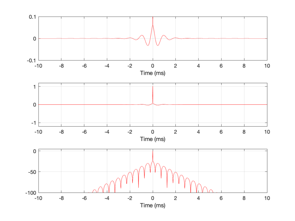
The top plot in Figure 4 is identical to the top plot in Figure 3. The middle plot is also on a linear amplitude scale, but the range of the plot shows the entire range of the signal. You can see there that the impulse at T = 0 hits a value of 1, and so the pre- and post-ringing isn’t as loud as you might have thought based on the first three figures.

The bottom plot shows the same information, plotted on a dB scale instead. The impulse at T = 0 ms hits 0 dB. Relative to that, the pre- and post-ringing has a maximum value of about -24 dB. You can also see there that the ringing is at least 100 dB down by the time we’re 6 ms away from the main impulse, looking both backwards and forwards in time.

Of course, all of these characteristics would be different for filters with different parameters. The point here is to understand the general characteristics, not the specifics.

Additional Comment

You may read on various fora someone who claims that there’s no such thing as “pre-ringing”. “It’s ‘ripple'” They’ll claim.

This is incorrect.

Pre-ringing and ringing are behaviours that occur in the time domain.

Ripple is a wiggle in the response in the frequency domain. (Say, for example, you zoom into the magnitude response, it won’t be completely flat in some cases – and if it’s not, you have ripple.)